The first type of self-balancing binary search tree to be invented is the AVL tree. The name AVL tree is coined after its inventor’s names − Adelson-Velsky and Landis.
In AVL trees, the difference between the heights of left and right subtrees, known as the Balance Factor, must be at most one. Once the difference exceeds one, the tree automatically executes the balancing algorithm until the difference becomes one again.
BALANCE FACTOR =
HEIGHT(LEFT SUBTREE) − HEIGHT(RIGHT SUBTREE)
There are usually four cases of rotation in the balancing algorithm of AVL trees: LL, RR, LR, RL.
LL Rotations
LL rotation is performed when the node is inserted into the right subtree leading to an unbalanced tree. This is a single left rotation to make the tree balanced again −
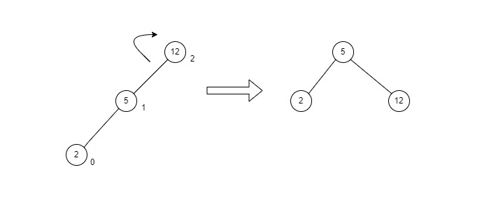
Fig : LL Rotation
The node where the unbalance occurs becomes the left child and the newly added node becomes the right child with the middle node as the parent node.
RR Rotations
RR rotation is performed when the node is inserted into the left subtree leading to an unbalanced tree. This is a single right rotation to make the tree balanced again −
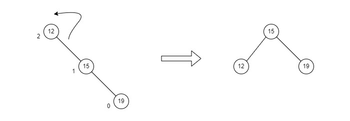
Fig : RR Rotation
The node where the unbalance occurs becomes the right child and the newly added node becomes the left child with the middle node as the parent node.
LR Rotations
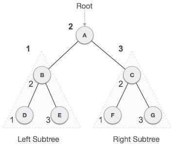
LR rotation is the extended version of the previous single rotations, also called a double rotation. It is performed when a node is inserted into the right subtree of the left subtree. The LR rotation is a combination of the left rotation followed by the right rotation. There are multiple steps to be followed to carry this out.
- Consider an example with A as the root node, B as the left child of A and C as the right child of B.
- Since the unbalance occurs at A, a left rotation is applied on the child nodes of A, i.e. B and C.
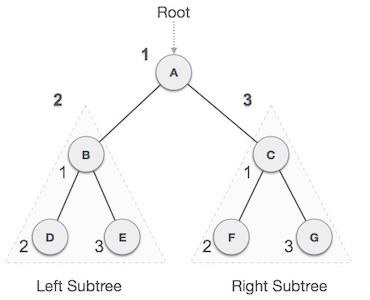
- After the rotation, the C node becomes the left child of A and B becomes the left child of C.
- The unbalance still persists, therefore a right rotation is applied at the root node A and the left child C.
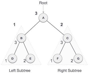
- After the final right rotation, C becomes the root node, A becomes the right child and B is the left child.
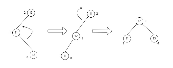
Fig : LR Rotation
RL Rotations
RL rotation is also the extended version of the previous single rotations, hence it is called a double rotation and it is performed if a node is inserted into the left subtree of the right subtree. The RL rotation is a combination of the right rotation followed by the left rotation. There are multiple steps to be followed to carry this out.
- Consider an example with A as the root node, B as the right child of A and C as the left child of B.
- Since the unbalance occurs at A, a right rotation is applied on the child nodes of A, i.e. B and C.
- After the rotation, the C node becomes the right child of A and B becomes the right child of C.
- The unbalance still persists, therefore a left rotation is applied at the root node A and the right child C.
- After the final left rotation, C becomes the root node, A becomes the left child and B is the right child.
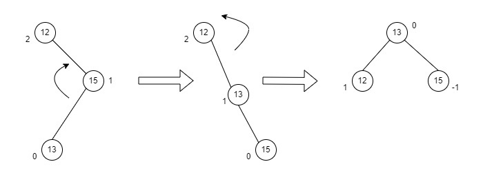
Fig : RL Rotation
Basic Operations of AVL Trees
The basic operations performed on the AVL Tree structures include all the operations performed on a binary search tree, since the AVL Tree at its core is actually just a binary search tree holding all its properties. Therefore, basic operations performed on an AVL Tree are − Insertion and Deletion.
Insertion operation
The data is inserted into the AVL Tree by following the Binary Search Tree property of insertion, i.e. the left subtree must contain elements less than the root value and right subtree must contain all the greater elements.
However, in AVL Trees, after the insertion of each element, the balance factor of the tree is checked; if it does not exceed 1, the tree is left as it is. But if the balance factor exceeds 1, a balancing algorithm is applied to readjust the tree such that balance factor becomes less than or equal to 1 again.Algorithm
The following steps are involved in performing the insertion operation of an AVL Tree −
Step 1 − Create a node
Step 2 − Check if the tree is empty
Step 3 − If the tree is empty, the new node created will become the
         root node of the AVL Tree.
Step 4 − If the tree is not empty, we perform the Binary Search Tree
         insertion operation and check the balancing factor of the node
         in the tree.
Step 5 − Suppose the balancing factor exceeds 1, we apply suitable
         rotations on the said node and resume the insertion from Step 4.
Let us understand the insertion operation by constructing an example AVL tree with 1 to 7 integers.
Starting with the first element 1, we create a node and measure the balance, i.e., 0.

Since both the binary search property and the balance factor are satisfied, we insert another element into the tree.
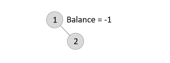
The balance factor for the two nodes are calculated and is found to be -1 (Height of left subtree is 0 and height of the right subtree is 1). Since it does not exceed 1, we add another element to the tree.
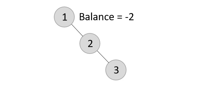
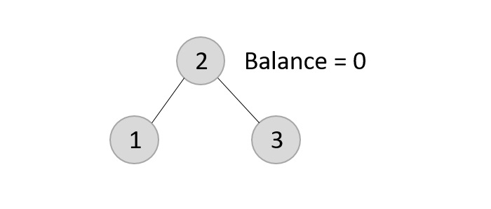
Now, after adding the third element, the balance factor exceeds 1 and becomes 2. Therefore, rotations are applied. In this case, the RR rotation is applied since the imbalance occurs at two right nodes.
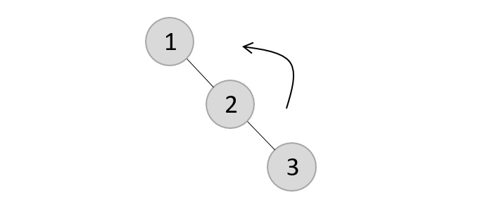
The tree is rearranged as −
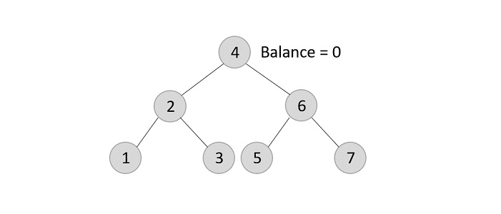
Similarly, the next elements are inserted and rearranged using these rotations. After rearrangement, we achieve the tree as −
Example
Following are the implementations of this operation in various programming languages −
#include <stdio.h>#include <stdlib.h>structNode{int data;structNode*leftChild;structNode*rightChild;int height;};intmax(int a,int b);intheight(structNode*N){if(N ==NULL)return0;return N->height;}intmax(int a,int b){return(a > b)? a : b;}structNode*newNode(int data){structNode*node =(structNode*)malloc(sizeof(structNode));
   node->data = data;
   node->leftChild =NULL;
   node->rightChild =NULL;
   node->height =1;return(node);}structNode*rightRotate(structNode*y){structNode*x = y->leftChild;structNode*T2 = x->rightChild;
   x->rightChild = y;
   y->leftChild = T2;
   y->height =max(height(y->leftChild),height(y->rightChild))+1;
   x->height =max(height(x->leftChild),height(x->rightChild))+1;return x;}structNode*leftRotate(structNode*x){structNode*y = x->rightChild;structNode*T2 = y->leftChild;
   y->leftChild = x;
   x->rightChild = T2;
   x->height =max(height(x->leftChild),height(x->rightChild))+1;
   y->height =max(height(y->leftChild),height(y->rightChild))+1;return y;}intgetBalance(structNode*N){if(N ==NULL)return0;returnheight(N->leftChild)-height(N->rightChild);}structNode*insertNode(structNode*node,int data){if(node ==NULL)return(newNode(data));if(data < node->data)
      node->leftChild =insertNode(node->leftChild, data);elseif(data > node->data)
      node->rightChild =insertNode(node->rightChild, data);elsereturn node;
   node->height =1+max(height(node->leftChild),height(node->rightChild));int balance =getBalance(node);if(balance >1&& data < node->leftChild->data)returnrightRotate(node);if(balance <-1&& data > node->rightChild->data)returnleftRotate(node);if(balance >1&& data > node->leftChild->data){
      node->leftChild =leftRotate(node->leftChild);returnrightRotate(node);}if(balance <-1&& data < node->rightChild->data){
      node->rightChild =rightRotate(node->rightChild);returnleftRotate(node);}return node;}structNode*minValueNode(structNode*node){structNode*current = node;while(current->leftChild !=NULL)
      current = current->leftChild;return current;}voidprintTree(structNode*root){if(root ==NULL)return;if(root !=NULL){printTree(root->leftChild);printf("%d ", root->data);printTree(root->rightChild);}}intmain(){structNode*root =NULL;
   root =insertNode(root,22);
   root =insertNode(root,14);
   root =insertNode(root,72);
   root =insertNode(root,44);
   root =insertNode(root,25);
   root =insertNode(root,63);
   root =insertNode(root,98);printf("AVL Tree: ");printTree(root);return0;}
Output
AVL Tree: 14 22 25 44 63 72 98
Deletion operation
Deletion in the AVL Trees take place in three different scenarios −
- Scenario 1 (Deletion of a leaf node) − If the node to be deleted is a leaf node, then it is deleted without any replacement as it does not disturb the binary search tree property. However, the balance factor may get disturbed, so rotations are applied to restore it.
- Scenario 2 (Deletion of a node with one child) − If the node to be deleted has one child, replace the value in that node with the value in its child node. Then delete the child node. If the balance factor is disturbed, rotations are applied.
- Scenario 3 (Deletion of a node with two child nodes) − If the node to be deleted has two child nodes, find the inorder successor of that node and replace its value with the inorder successor value. Then try to delete the inorder successor node. If the balance factor exceeds 1 after deletion, apply balance algorithms.
Using the same tree given above, let us perform deletion in three scenarios −
- Deleting element 7 from the tree above −
Since the element 7 is a leaf, we normally remove the element without disturbing any other node in the tree
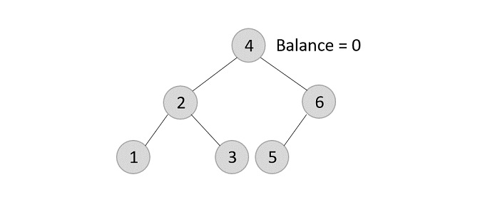
- Deleting element 6 from the output tree achieved −
However, element 6 is not a leaf node and has one child node attached to it. In this case, we replace node 6 with its child node: node 5.
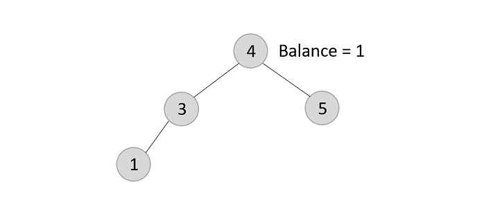
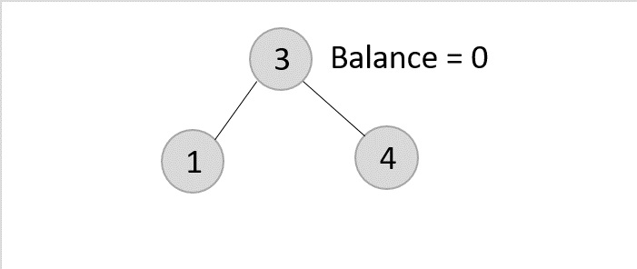
The balance of the tree becomes 1, and since it does not exceed 1 the tree is left as it is. If we delete the element 5 further, we would have to apply the left rotations; either LL or LR since the imbalance occurs at both 1-2-4 and 3-2-4.
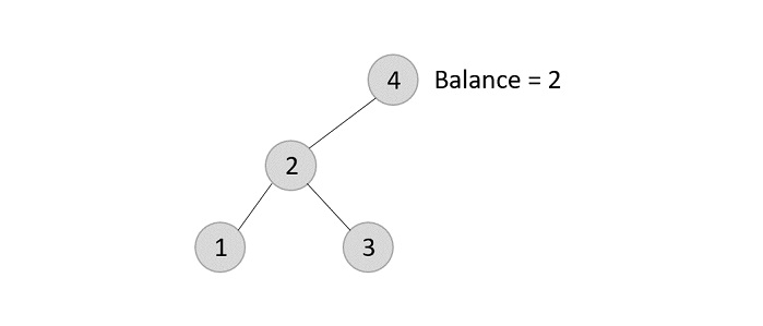
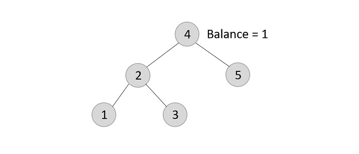
The balance factor is disturbed after deleting the element 5, therefore we apply LL rotation (we can also apply the LR rotation here).
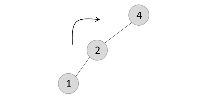
Once the LL rotation is applied on path 1-2-4, the node 3 remains as it was supposed to be the right child of node 2 (which is now occupied by node 4). Hence, the node is added to the right subtree of the node 2 and as the left child of the node 4.
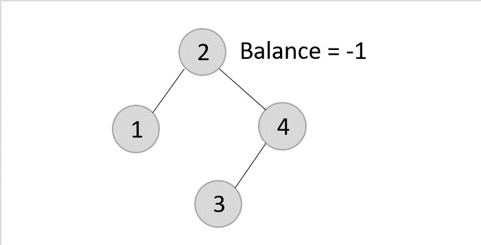
- Deleting element 2 from the remaining tree −
As mentioned in scenario 3, this node has two children. Therefore, we find its inorder successor that is a leaf node (say, 3) and replace its value with the inorder successor.
The balance of the tree still remains 1, therefore we leave the tree as it is without performing any rotations.Example
Following are the implementations of this operation in various programming languages −
#include <stdio.h>#include <stdlib.h>structNode{int data;structNode*leftChild;structNode*rightChild;int height;};intmax(int a,int b);intheight(structNode*N){if(N ==NULL)return0;return N->height;}intmax(int a,int b){return(a > b)? a : b;}structNode*newNode(int data){structNode*node =(structNode*)malloc(sizeof(structNode));
   node->data = data;
   node->leftChild =NULL;
   node->rightChild =NULL;
   node->height =1;return(node);}structNode*rightRotate(structNode*y){structNode*x = y->leftChild;structNode*T2 = x->rightChild;
   x->rightChild = y;
   y->leftChild = T2;
   y->height =max(height(y->leftChild),height(y->rightChild))+1;
   x->height =max(height(x->leftChild),height(x->rightChild))+1;return x;}structNode*leftRotate(structNode*x){structNode*y = x->rightChild;structNode*T2 = y->leftChild;
   y->leftChild = x;
   x->rightChild = T2;
   x->height =max(height(x->leftChild),height(x->rightChild))+1;
   y->height =max(height(y->leftChild),height(y->rightChild))+1;return y;}intgetBalance(structNode*N){if(N ==NULL)return0;returnheight(N->leftChild)-height(N->rightChild);}structNode*insertNode(structNode*node,int data){if(node ==NULL)return(newNode(data));if(data < node->data)
      node->leftChild =insertNode(node->leftChild, data);elseif(data > node->data)
      node->rightChild =insertNode(node->rightChild, data);elsereturn node;
   node->height =1+max(height(node->leftChild),height(node->rightChild));int balance =getBalance(node);if(balance >1&& data < node->leftChild->data)returnrightRotate(node);if(balance <-1&& data > node->rightChild->data)returnleftRotate(node);if(balance >1&& data > node->leftChild->data){
      node->leftChild =leftRotate(node->leftChild);returnrightRotate(node);}if(balance <-1&& data < node->rightChild->data){
      node->rightChild =rightRotate(node->rightChild);returnleftRotate(node);}return node;}structNode*minValueNode(structNode*node){structNode*current = node;while(current->leftChild !=NULL)
      current = current->leftChild;return current;}structNode*deleteNode(structNode*root,int data){if(root ==NULL)return root;if(data < root->data)
      root->leftChild =deleteNode(root->leftChild, data);elseif(data > root->data)
      root->rightChild =deleteNode(root->rightChild, data);else{if((root->leftChild ==NULL)||(root->rightChild ==NULL)){structNode*temp = root->leftChild ? root->leftChild : root->rightChild;if(temp ==NULL){
            temp = root;
            root =NULL;}else*root =*temp;free(temp);}else{structNode*temp =minValueNode(root->rightChild);
         root->data = temp->data;
         root->rightChild =deleteNode(root->rightChild, temp->data);}}if(root ==NULL)return root;
   root->height =1+max(height(root->leftChild),height(root->rightChild));int balance =getBalance(root);if(balance >1&&getBalance(root->leftChild)>=0)returnrightRotate(root);if(balance >1&&getBalance(root->leftChild)<0){
      root->leftChild =leftRotate(root->leftChild);returnrightRotate(root);}if(balance <-1&&getBalance(root->rightChild)<=0)returnleftRotate(root);if(balance <-1&&getBalance(root->rightChild)>0){
      root->rightChild =rightRotate(root->rightChild);returnleftRotate(root);}return root;}// Print the treevoidprintTree(structNode*root){if(root !=NULL){printTree(root->leftChild);printf("%d ", root->data);printTree(root->rightChild);}}intmain(){structNode*root =NULL;
   root =insertNode(root,22);
   root =insertNode(root,14);
   root =insertNode(root,72);
   root =insertNode(root,44);
   root =insertNode(root,25);
   root =insertNode(root,63);
   root =insertNode(root,98);printf("AVL Tree: ");printTree(root);
   root =deleteNode(root,25);printf("\nAfter deletion: ");printTree(root);return0;}
Output
AVL Tree: 14 22 25 44 63 72 98
After deletion: 14 22 44 63 72 98