Among all the algorithmic approaches, the simplest and straightforward approach is the Greedy method. In this approach, the decision is taken on the basis of current available information without worrying about the effect of the current decision in future.
Greedy algorithms build a solution part by part, choosing the next part in such a way, that it gives an immediate benefit. This approach never reconsiders the choices taken previously. This approach is mainly used to solve optimization problems. Greedy method is easy to implement and quite efficient in most of the cases. Hence, we can say that Greedy algorithm is an algorithmic paradigm based on heuristic that follows local optimal choice at each step with the hope of finding global optimal solution.
In many problems, it does not produce an optimal solution though it gives an approximate (near optimal) solution in a reasonable time.
Components of Greedy Algorithm
Greedy algorithms have the following five components −
A candidate set − A solution is created from this set.
A selection function − Used to choose the best candidate to be added to the solution.
A feasibility function − Used to determine whether a candidate can be used to contribute to the solution.
An objective function − Used to assign a value to a solution or a partial solution.
A solution function − Used to indicate whether a complete solution has been reached.
Areas of Application
Greedy approach is used to solve many problems, such as
Finding the shortest path between two vertices using Dijkstra’s algorithm.
Finding the minimal spanning tree in a graph using Prim’s /Kruskal’s algorithm, etc.
Counting Coins Problem
The Counting Coins problem is to count to a desired value by choosing the least possible coins and the greedy approach forces the algorithm to pick the largest possible coin. If we are provided coins of 1, 2, 5 and 10 and we are asked to count 18 then the greedy procedure will be −
1 − Select one 10 coin, the remaining count is 8
2 − Then select one 5 coin, the remaining count is 3
3 − Then select one 2 coin, the remaining count is 1
4 − And finally, the selection of one 1 coins solves the problem
Though, it seems to be working fine, for this count we need to pick only 4 coins. But if we slightly change the problem then the same approach may not be able to produce the same optimum result.
For the currency system, where we have coins of 1, 7, 10 value, counting coins for value 18 will be absolutely optimum but for count like 15, it may use more coins than necessary. For example, the greedy approach will use 10 + 1 + 1 + 1 + 1 + 1, total 6 coins. Whereas the same problem could be solved by using only 3 coins (7 + 7 + 1)
Hence, we may conclude that the greedy approach picks an immediate optimized solution and may fail where global optimization is a major concern.
Where Greedy Approach Fails
In many problems, Greedy algorithm fails to find an optimal solution, moreover it may produce a worst solution. Problems like Travelling Salesman and Knapsack cannot be solved using this approach.
Examples of Greedy Algorithm
Most networking algorithms use the greedy approach. Here is a list of few of them −
Travelling Salesman Problem
Prim’s Minimal Spanning Tree Algorithm
Kruskal’s Minimal Spanning Tree Algorithm
Dijkstra’s Minimal Spanning Tree Algorithm
Graph − Map Coloring
Graph − Vertex Cover
DSA – Fractional Knapsack Problem
DSA – Job Sequencing with Deadline
DSA – Optimal Merge Pattern Algorithm
We will discuss these examples elaborately in the further chapters of this tutorial.
The Karatsuba algorithm is used by the system to perform fast multiplication on two n-digit numbers, i.e. the system compiler takes lesser time to compute the product than the time-taken by a normal multiplication.
The usual multiplication approach takes n2 computations to achieve the final product, since the multiplication has to be performed between all digit combinations in both the numbers and then the sub-products are added to obtain the final product. This approach of multiplication is known as Naive Multiplication.
To understand this multiplication better, let us consider two 4-digit integers: 1456 and 6533, and find the product using Naive approach.
So, 1456 6533 =?
In this method of naive multiplication, given the number of digits in both numbers is 4, there are 16 single-digit single-digit multiplications being performed. Thus, the time complexity of this approach is O(42) since it takes 42 steps to calculate the final product.
But when the value of n keeps increasing, the time complexity of the problem also keeps increasing. Hence, Karatsuba algorithm is adopted to perform faster multiplications.
Karatsuba Algorithm
The main idea of the Karatsuba Algorithm is to reduce multiplication of multiple sub problems to multiplication of three sub problems. Arithmetic operations like additions and subtractions are performed for other computations.
For this algorithm, two n-digit numbers are taken as the input and the product of the two number is obtained as the output.
Step 1 − In this algorithm we assume that n is a power of 2.
Step 2 − If n = 1 then we use multiplication tables to find P = XY.
Step 3 − If n > 1, the n-digit numbers are split in half and represent the number using the formulae −
X = 10n/2X1 + X2
Y = 10n/2Y1 + Y2
where, X1, X2, Y1, Y2 each have n/2 digits.
Step 4 − Take a variable Z = W (U + V),
where,
U = X1Y1, V = X2Y2
W = (X1 + X2) (Y1 + Y2), Z = X1Y2 + X2Y1.
Step 5 − Then, the product P is obtained after substituting the values in the formula −
P = 10n(U) + 10n/2(Z) + V
P = 10n (X1Y1) + 10n/2 (X1Y2 + X2Y1) + X2Y2.
Step 6 − Recursively call the algorithm by passing the sub problems (X1, Y1), (X2, Y2) and (X1 + X2, Y1 + Y2) separately. Store the returned values in variables U, V and W respectively.
Example
Let us solve the same problem given above using Karatsuba method, 1456 6533 −
The Karatsuba method takes the divide and conquer approach by dividing the problem into multiple sub-problems and applies recursion to make the multiplication simpler.
Step 1
Assuming that n is the power of 2, rewrite the n-digit numbers in the form of −
X = 10n/2X1 + X2 Y = 10n/2Y1 + Y2
That gives us,
1456 = 102(14) + 56
6533 = 102(65) + 33
First let us try simplifying the mathematical expression, we get,
The above expression is the simplified version of the given multiplication problem, since multiplying two double-digit numbers can be easier to solve rather than multiplying two four-digit numbers.
However, that holds true for the human mind. But for the system compiler, the above expression still takes the same time complexity as the normal naive multiplication. Since it has 4 double-digit double-digit multiplications, the time complexity taken would be −
U = 910
V = 1848
Z = W  (U + V) = 6860  (1848 + 910) = 4102
Substituting the values in equation,
P = 10n. U + 10n/2. Z + V
P = 104 (910) + 102 (4102) + 1848
P = 91,00,000 + 4,10,200 + 1848
P = 95,12,048
Analysis
The Karatsuba algorithm is a recursive algorithm; since it calls smaller instances of itself during execution.
According to the algorithm, it calls itself only thrice on n/2-digit numbers in order to achieve the final product of two n-digit numbers.
Now, if T(n) represents the number of digit multiplications required while performing the multiplication,
T(n) = 3T(n/2)
This equation is a simple recurrence relation which can be solved as −
Apply T(n/2) = 3T(n/4) in the above equation, we get:
T(n) = 9T(n/4)
T(n) = 27T(n/8)
T(n) = 81T(n/16)
.
.
.
.
T(n) = 3i T(n/2i) is the general form of the recurrence relation
of Karatsuba algorithm.
Recurrence relations can be solved using the masters theorem, since we have a dividing function in the form of −
T(n) = aT(n/b) + f(n), where, a = 3, b = 2 and f(n) = 0
which leads to k = 0.
Since f(n) represents work done outside the recursion, which are addition and subtraction arithmetic operations in Karatsuba, these arithmetic operations do not contribute to time complexity.
Check the relation between a and bk.
a > bk = 3 > 20
According to masters theorem, apply case 1.
T(n) = O(nlogb a)
T(n) = O(nlog 3)
The time complexity of Karatsuba algorithm for fast multiplication is O(nlog 3).
Example
In the complete implementation of Karatsuba Algorithm, we are trying to multiply two higher-valued numbers. Here, since the long data type accepts decimals upto 18 places, we take the inputs as long values. The Karatsuba function is called recursively until the final product is obtained.
#include <stdio.h>#include <math.h>intget_size(long);longkaratsuba(long X,long Y){// Base Caseif(X <10&& Y <10)return X * Y;// determine the size of X and Yint size =fmax(get_size(X),get_size(Y));if(size <10)return X * Y;// rounding up the max length
   size =(size/2)+(size%2);long multiplier =pow(10, size);long b = X/multiplier;long a = X -(b * multiplier);long d = Y / multiplier;long c = Y -(d * size);long u =karatsuba(a, c);long z =karatsuba(a + b, c + d);long v =karatsuba(b, d);return u +((z - u - v)* multiplier)+(v *(long)(pow(10,2* size)));}intget_size(long value){int count =0;while(value >0){
      count++;
      value /=10;}return count;}intmain(){// two numberslong x =145623;long y =653324;printf("The final product is: %ld\n",karatsuba(x, y));return0;}
Strassen’s Matrix Multiplication is the divide and conquer approach to solve the matrix multiplication problems. The usual matrix multiplication method multiplies each row with each column to achieve the product matrix. The time complexity taken by this approach is O(n3), since it takes two loops to multiply. Strassens method was introduced to reduce the time complexity from O(n3) to O(nlog 7).
Naive Method
First, we will discuss Naive method and its complexity. Here, we are calculating Z=X Y. Using Naive method, two matrices (X and Y) can be multiplied if the order of these matrices are pq and qr and the resultant matrix will be of order pr. The following pseudocode describes the Naive multiplication −
Algorithm: Matrix-Multiplication (X, Y, Z)
for i = 1 to p do
   for j = 1 to r do
      Z[i,j] := 0
      for k = 1 to q do
         Z[i,j] := Z[i,j] + X[i,k] × Y[k,j]
Complexity
Here, we assume that integer operations take O(1) time. There are three for loops in this algorithm and one is nested in other. Hence, the algorithm takes O(n3) time to execute.
Strassens Matrix Multiplication Algorithm
In this context, using Strassens Matrix multiplication algorithm, the time consumption can be improved a little bit.
Strassens Matrix multiplication can be performed only on square matrices where n is a power of 2. Order of both of the matrices are n × n.
Divide X, Y and Z into four (n/2)×(n/2) matrices as represented below −
Let us consider a simple problem that can be solved by divide and conquer technique.
Max-Min Problem
The Max-Min Problem in algorithm analysis is finding the maximum and minimum value in an array.
Solution
To find the maximum and minimum numbers in a given array numbers[] of size n, the following algorithm can be used. First we are representing the naive method and then we will present divide and conquer approach.
Naive Method
Naive method is a basic method to solve any problem. In this method, the maximum and minimum number can be found separately. To find the maximum and minimum numbers, the following straightforward algorithm can be used.
Algorithm: Max-Min-Element (numbers[])
max := numbers[1]
min := numbers[1]

for i = 2 to n do
   if numbers[i] > max then
      max := numbers[i]
   if numbers[i] < min then
      min := numbers[i]
return (max, min)
Example
Following are the implementations of the above approach in various programming languages −
#include <stdio.h>structPair{int max;int min;};// Function to find maximum and minimum using the naive algorithmstructPairmaxMinNaive(int arr[],int n){structPair result;
    result.max = arr[0];
    result.min = arr[0];// Loop through the array to find the maximum and minimum valuesfor(int i =1; i < n; i++){if(arr[i]> result.max){
            result.max = arr[i];// Update the maximum value if a larger element is found}if(arr[i]< result.min){
            result.min = arr[i];// Update the minimum value if a smaller element is found}}return result;// Return the pair of maximum and minimum values}intmain(){int arr[]={6,4,26,14,33,64,46};int n =sizeof(arr)/sizeof(arr[0]);structPair result =maxMinNaive(arr, n);printf("Maximum element is: %d\n", result.max);printf("Minimum element is: %d\n", result.min);return0;}
Output
Maximum element is: 64
Minimum element is: 4
Analysis
The number of comparison in Naive method is 2n – 2.
The number of comparisons can be reduced using the divide and conquer approach. Following is the technique.
Divide and Conquer Approach
In this approach, the array is divided into two halves. Then using recursive approach maximum and minimum numbers in each halves are found. Later, return the maximum of two maxima of each half and the minimum of two minima of each half.
In this given problem, the number of elements in an array is y−x+1, where y is greater than or equal to x.
Max−Min(x,y) will return the maximum and minimum values of an array numbers[x…y].
Algorithm: Max - Min(x, y)
if y  x ≤ 1 then
   return (max(numbers[x],numbers[y]),min((numbers[x],numbers[y]))
else
   (max1, min1):= maxmin(x, ⌊((x + y)/2)⌋)
   (max2, min2):= maxmin(⌊((x + y)/2) + 1)⌋,y)
return (max(max1, max2), min(min1, min2))
Example
Following are implementations of the above approach in various programming languages −
#include <stdio.h>// Structure to store both maximum and minimum elementsstructPair{int max;int min;};structPairmaxMinDivideConquer(int arr[],int low,int high){structPair result;structPair left;structPair right;int mid;// If only one element in the arrayif(low == high){
        result.max = arr[low];
        result.min = arr[low];return result;}// If there are two elements in the arrayif(high == low +1){if(arr[low]< arr[high]){
            result.min = arr[low];
            result.max = arr[high];}else{
            result.min = arr[high];
            result.max = arr[low];}return result;}// If there are more than two elements in the array
    mid =(low + high)/2;
    left =maxMinDivideConquer(arr, low, mid);
    right =maxMinDivideConquer(arr, mid +1, high);// Compare and get the maximum of both parts
    result.max =(left.max > right.max)? left.max : right.max;// Compare and get the minimum of both parts
    result.min =(left.min < right.min)? left.min : right.min;return result;}intmain(){int arr[]={6,4,26,14,33,64,46};int n =sizeof(arr)/sizeof(arr[0]);structPair result =maxMinDivideConquer(arr,0, n -1);printf("Maximum element is: %d\n", result.max);printf("Minimum element is: %d\n", result.min);return0;}
Output
Maximum element is: 64
Minimum element is: 4
Analysis
Let T(n) be the number of comparisons made by Max−Min(x,y), where the number of elements n=y−x+1.
If T(n) represents the numbers, then the recurrence relation can be represented as
T(n)=⎧⎩⎨⎪⎪T(⌊n2⌋)+T(⌈n2⌉)+210forn>2forn=2forn=1
Let us assume that n is in the form of power of 2. Hence, n = 2k where k is height of the recursion tree.
So,
T(n)=2.T(n2)+2=2.(2.T(n4)+2)+2…..=3n2−2
Compared to Nave method, in divide and conquer approach, the number of comparisons is less. However, using the asymptotic notation both of the approaches are represented by O(n).
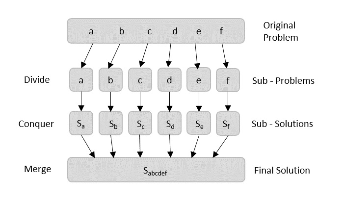
Using divide and conquer approach, the problem in hand, is divided into smaller sub-problems and then each problem is solved independently. When we keep dividing the sub-problems into even smaller sub-problems, we may eventually reach a stage where no more division is possible. Those smallest possible sub-problems are solved using original solution because it takes lesser time to compute. The solution of all sub-problems is finally merged in order to obtain the solution of the original problem.
Broadly, we can understand divide-and-conquer approach in a three-step process.
Divide/Break
This step involves breaking the problem into smaller sub-problems. Sub-problems should represent a part of the original problem. This step generally takes a recursive approach to divide the problem until no sub-problem is further divisible. At this stage, sub-problems become atomic in size but still represent some part of the actual problem.
Conquer/Solve
This step receives a lot of smaller sub-problems to be solved. Generally, at this level, the problems are considered ‘solved’ on their own.
Merge/Combine
When the smaller sub-problems are solved, this stage recursively combines them until they formulate a solution of the original problem. This algorithmic approach works recursively and conquer & merge steps works so close that they appear as one.
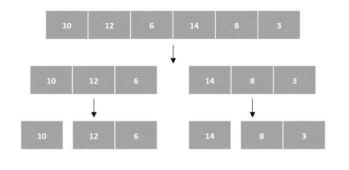
Arrays as Input
There are various ways in which various algorithms can take input such that they can be solved using the divide and conquer technique. Arrays are one of them. In algorithms that require input to be in the form of a list, like various sorting algorithms, array data structures are most commonly used.
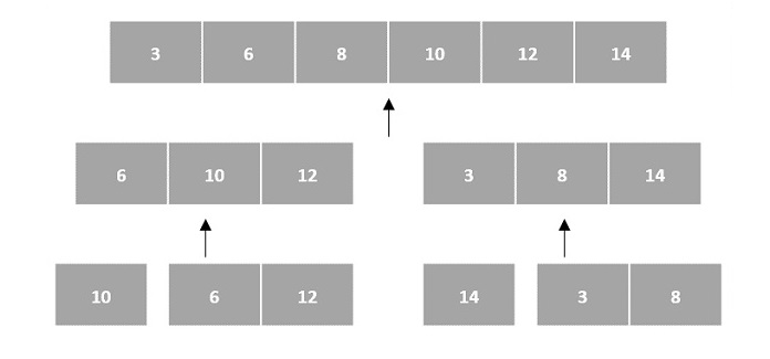
In the input for a sorting algorithm below, the array input is divided into subproblems until they cannot be divided further.
Then, the subproblems are sorted (the conquer step) and are merged to form the solution of the original array back (the combine step).
Since arrays are indexed and linear data structures, sorting algorithms most popularly use array data structures to receive input.
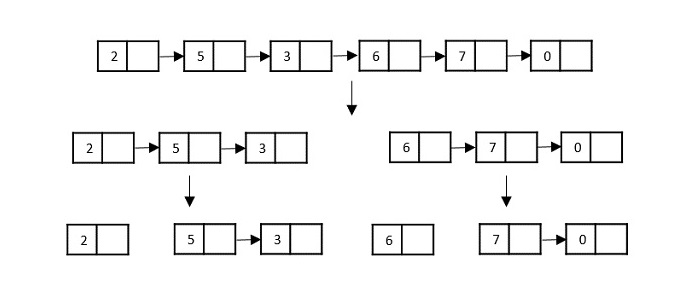
Linked Lists as Input
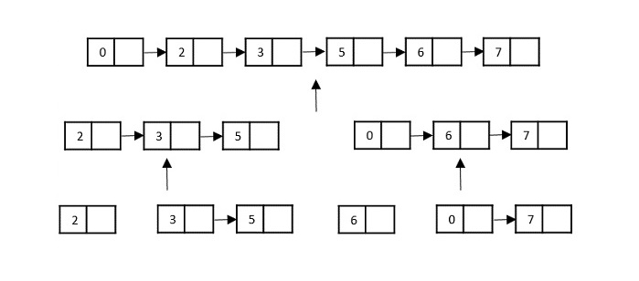
Another data structure that can be used to take input for divide and conquer algorithms is a linked list (for example, merge sort using linked lists). Like arrays, linked lists are also linear data structures that store data sequentially.
Consider the merge sort algorithm on linked list; following the very popular tortoise and hare algorithm, the list is divided until it cannot be divided further.
Then, the nodes in the list are sorted (conquered). These nodes are then combined (or merged) in recursively until the final solution is achieved.
Various searching algorithms can also be performed on the linked list data structures with a slightly different technique as linked lists are not indexed linear data structures. They must be handled using the pointers available in the nodes of the list.
Pros and cons of Divide and Conquer Approach
Divide and conquer approach supports parallelism as sub-problems are independent. Hence, an algorithm, which is designed using this technique, can run on the multiprocessor system or in different machines simultaneously.
In this approach, most of the algorithms are designed using recursion, hence memory management is very high. For recursive function stack is used, where function state needs to be stored.
Examples of Divide and Conquer Approach
The following computer algorithms are based on divide-and-conquer programming approach −
Fibonacci series generates the subsequent number by adding two previous numbers. Fibonacci series starts from two numbers F0 & F1. The initial values of F0 & F1 can be taken 0, 1 or 1, 1 respectively.
Fibonacci series satisfies the following conditions −
Fn = Fn-1 + Fn-2
Hence, a Fibonacci series can look like this −
F8 = 0 1 1 2 3 5 8 13
or, this −
F8 = 1 1 2 3 5 8 13 21
For illustration purpose, Fibonacci of F8 is displayed as −
Fibonacci Iterative Algorithm
First we try to draft the iterative algorithm for Fibonacci series.
Procedure Fibonacci(n)
declare f0, f1, fib, loop
set f0 to 0
set f1 to 1<b>display f0, f1</b>for loop ← 1 to n
fib ← f0 + f1
f0 ← f1
f1 ← fib
<b>display fib</b>
end for
end procedure
Fibonacci Recursive Algorithm
Let us learn how to create a recursive algorithm Fibonacci series. The base criteria of recursion.
START
Procedure Fibonacci(n)
   declare f0, f1, fib, loop

   set f0 to 0
   set f1 to 1

   display f0, f1

   for loop ← 1 to n

      fib ← f0 + f1
      f0 ← f1
      f1 ← fib

      display fib
   end for

END
Example
Following are the implementations of the above approach in various programming languages −
#include <stdio.h>intfibbonacci(int n){if(n ==0){return0;}elseif(n ==1){return1;}else{return(fibbonacci(n-1)+fibbonacci(n-2));}}intmain(){int n =5;printf("Number is: %d", n);printf("\nFibonacci series upto number %d are: ", n);for(int i =0;i<n;i++){printf("%d ",fibbonacci(i));}}
Output
Number is: 5
Fibonacci series upto number 5 are: 0 1 1 2 3
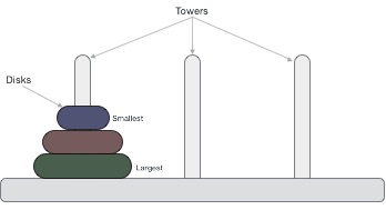
Tower of Hanoi, is a mathematical puzzle which consists of three towers (pegs) and more than one rings is as depicted −
These rings are of different sizes and stacked upon in an ascending order, i.e. the smaller one sits over the larger one. There are other variations of the puzzle where the number of disks increase, but the tower count remains the same.
Rules
The mission is to move all the disks to some another tower without violating the sequence of arrangement. A few rules to be followed for Tower of Hanoi are −
Only one disk can be moved among the towers at any given time.
Only the “top” disk can be removed.
No large disk can sit over a small disk.
Following is an animated representation of solving a Tower of Hanoi puzzle with three disks.
Tower of Hanoi puzzle with n disks can be solved in minimum 2n−1 steps. This presentation shows that a puzzle with 3 disks has taken 23 – 1 = 7 steps.
Algorithm
To write an algorithm for Tower of Hanoi, first we need to learn how to solve this problem with lesser amount of disks, say → 1 or 2. We mark three towers with name, source, destination and aux (only to help moving the disks). If we have only one disk, then it can easily be moved from source to destination peg.
If we have 2 disks −
First, we move the smaller (top) disk to aux peg.
Then, we move the larger (bottom) disk to destination peg.
And finally, we move the smaller disk from aux to destination peg.
So now, we are in a position to design an algorithm for Tower of Hanoi with more than two disks. We divide the stack of disks in two parts. The largest disk (nth disk) is in one part and all other (n-1) disks are in the second part.
Our ultimate aim is to move disk n from source to destination and then put all other (n1) disks onto it. We can imagine to apply the same in a recursive way for all given set of disks.
The steps to follow are −
Step 1 − Move n-1 disks from source to aux
Step 2 − Move nth disk from source to dest
Step 3 − Move n-1 disks from aux to dest
A recursive algorithm for Tower of Hanoi can be driven as follows −
START
Procedure Hanoi(disk, source, dest, aux)

   IF disk == 1, THEN
      move disk from source to dest
   ELSE
      Hanoi(disk - 1, source, aux, dest)     // Step 1
      move disk from source to dest          // Step 2
      Hanoi(disk - 1, aux, dest, source)     // Step 3
   END IF

END Procedure
STOP
Example
Following are the implementations of this approach in various programming languages −
#include <stdio.h>voidhanoi(int n,char from,char to,char via){if(n ==1){printf("Move disk 1 from %c to %c\n", from, to);}else{hanoi(n-1, from, via, to);printf("Move disk %d from %c to %c\n", n, from, to);hanoi(n-1, via, to, from);}}intmain(){int n =3;char from ='A';char to ='B';char via ='C';//calling hanoi() methodhanoi(n, from, via, to);}
Output
Move disk 1 from A to C
Move disk 2 from A to B
Move disk 1 from C to B
Move disk 3 from A to C
Move disk 1 from B to A
Move disk 2 from B to C
Move disk 1 from A to C
Some computer programming languages allow a module or function to call itself. This technique is known as recursion. In recursion, a function α either calls itself directly or calls a function β that in turn calls the original function α. The function α is called recursive function.
A recursive function can go infinite like a loop. To avoid infinite running of recursive function, there are two properties that a recursive function must have −
Base criteria − There must be at least one base criteria or condition, such that, when this condition is met the function stops calling itself recursively.
Progressive approach − The recursive calls should progress in such a way that each time a recursive call is made it comes closer to the base criteria.
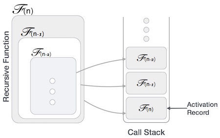
Implementation
Many programming languages implement recursion by means of stacks. Generally, whenever a function (caller) calls another function (callee) or itself as callee, the caller function transfers execution control to the callee. This transfer process may also involve some data to be passed from the caller to the callee.
This implies, the caller function has to suspend its execution temporarily and resume later when the execution control returns from the callee function. Here, the caller function needs to start exactly from the point of execution where it puts itself on hold. It also needs the exact same data values it was working on. For this purpose, an activation record (or stack frame) is created for the caller function.
This activation record keeps the information about local variables, formal parameters, return address and all information passed to the caller function.
Analysis of Recursion
One may argue why to use recursion, as the same task can be done with iteration. The first reason is, recursion makes a program more readable and because of latest enhanced CPU systems, recursion is more efficient than iterations.
Time Complexity
In case of iterations, we take number of iterations to count the time complexity. Likewise, in case of recursion, assuming everything is constant, we try to figure out the number of times a recursive call is being made. A call made to a function is Ο(1), hence the (n) number of times a recursive call is made makes the recursive function Ο(n).
Space Complexity
Space complexity is counted as what amount of extra space is required for a module to execute. In case of iterations, the compiler hardly requires any extra space. The compiler keeps updating the values of variables used in the iterations. But in case of recursion, the system needs to store activation record each time a recursive call is made. Hence, it is considered that space complexity of recursive function may go higher than that of a function with iteration.
Example
Following are the implementations of the recursion in various programming languages −
// C program for Recursion Data Structure#include <stdio.h>intfactorial(int n){// Base case: factorial of 0 is 1if(n ==0)return1;// Recursive case: multiply n with factorial of (n-1)return n *factorial(n -1);}intmain(){// case 1int number =6;printf("Number is: %d\n",6);//case 2if(number <0){printf("Error: Factorial is undefined for negative numbers.\n");return1;}int result =factorial(number);//print the outputprintf("Factorial of %d is: %d\n", number, result);return0;}
Priority search tree is a hybrid data structures, means it is a combination of binary search tree and priority queue. It is used for storing a set of points in a two-dimensional space, which are ordered by their priority and also key value.
It is a data structure that stores the points in sorted order based on their x-coordinate. Each node in the tree contains a priority queue that stores the points in sorted order based on their y-coordinate.
This data structure mainly used for solving the 2-D range query problem in computational geometry.
Structure of Priority Search Tree
Priority search tree has two main components:
Binary Search Tree: The binary search tree stores the points in sorted order based on their x-coordinate.The left subtree of a node contains points with x-coordinates less than the x-coordinate of the node, and the right subtree contains points with x-coordinates greater than the x-coordinate of the node.
Priority Queue: The priority queue stores the points in sorted order based on their y-coordinate.Each node in the tree contains a priority queue that stores the points in sorted order based on their y-coordinate.
Operations on Priority Search Tree
Priority search tree supports the following operations −
Insert: Insert a point into the priority search tree.
Search: Search for a point in the priority search tree based on its x-coordinate.
Range Query: Find all the points that lie within a given range in the two-dimensional space.
Implementing Priority Search Tree
Priority search tree can be implemented using a binary search tree and a priority queue.
Here is an example of a priority search tree implemented using a binary search tree and a priority queue:
#include <stdio.h>#include <stdlib.h>// Structure to represent a point in 2D spacestructPoint{int x, y;};// Structure to represent a node in the priority search treestructNode{structPoint point;structNode* left;structNode* right;};// Function to create a new nodestructNode*createNode(structPoint point){structNode* newNode =(structNode*)malloc(sizeof(structNode));
   newNode->point = point;
   newNode->left =NULL;
   newNode->right =NULL;return newNode;}// Function to insert a point into the priority search treestructNode*insert(structNode* root,structPoint point){if(root ==NULL){returncreateNode(point);}if(point.x < root->point.x){
       root->left =insert(root->left, point);}else{
       root->right =insert(root->right, point);}return root;}// Function to print the points in the priority search treevoidprintPoints(structNode* root){if(root !=NULL){printPoints(root->left);printf("(%d, %d) ", root->point.x, root->point.y);printPoints(root->right);}}intmain(){structNode* root =NULL;structPoint points[]={{5,3},{2,8},{9,1},{7,4},{3,6}};int n =sizeof(points)/sizeof(points[0]);for(int i =0; i < n; i++){
       root =insert(root, points[i]);}printf("Points in the priority search tree: ");printPoints(root);printf("\n");return0;}
Output
Output of the above code will be:
Points in the priority search tree: (2, 8) (3, 6) (5, 3) (7, 4) (9, 1)
Search in Priority Search Tree
Searching for a point in a priority search tree is similar to searching for a key in a binary search tree. We start at the root of the tree and recursively search the tree based on the x-coordinate of the point.
Let us understand how the search operation works in a priority search tree:
Algorithm
Following is the algorithm, follow the steps:
1. Start at the root of the tree.
2. return the root if it is null or the x-coordinate of the root is equal to the search key.
3. if the search key is less than the x-coordinate of the root, recursively search the left subtree.
4. if the search key is greater than the x-coordinate of the root, recursively search the right subtree.
5. return the node if found, otherwise return null.
Example code
Here is an example code that demonstrates the search operation in a priority search tree:
#include <stdio.h>#include <stdlib.h>// Structure to represent a point in 2D spacestructPoint{int x, y;};// Structure to represent a node in the priority search treestructNode{structPoint point;structNode* left;structNode* right;};// Function to create a new nodestructNode*createNode(structPoint point){structNode* newNode =(structNode*)malloc(sizeof(structNode));
   newNode->point = point;
   newNode->left =NULL;
   newNode->right =NULL;return newNode;}// Function to insert a point into the priority search treestructNode*insert(structNode* root,structPoint point){if(root ==NULL){returncreateNode(point);}if(point.x < root->point.x){
       root->left =insert(root->left, point);}else{
       root->right =insert(root->right, point);}return root;}// Function to search for a point in the priority search treestructNode*search(structNode* root,int x){if(root ==NULL|| root->point.x == x){return root;}if(x < root->point.x){returnsearch(root->left, x);}else{returnsearch(root->right, x);}}intmain(){structNode* root =NULL;structPoint points[]={{5,3},{2,8},{9,1},{7,4},{3,6}};int n =sizeof(points)/sizeof(points[0]);for(int i =0; i < n; i++){
       root =insert(root, points[i]);}int x =7;structNode* result =search(root, x);if(result !=NULL){printf("Point with x-coordinate %d found: (%d, %d)\n", x, result->point.x, result->point.y);}else{printf("Point with x-coordinate %d not found\n", x);}return0;}
Output
Output of the above code will be:
Point with x-coordinate 7 found: (7, 4)
Range Query in Priority Search Tree
This operation is the main application of the priority search tree. It is used to find all the points that lie within a given range in the two-dimensional space.
Algorithm
Following is the algorithm, follow the steps:
1. Start at the root of the tree.
2. If the range intersects the x-coordinate of the node, search the priority queue at the node based on the y-coordinate of the range.
3. Retrieve the points that lie within the range.
4. Recursively search the left and right subtrees based on the x-coordinate of the range.
5. Return the points that lie within the range.
Example code
Here is an example code that demonstrates the range query operation in a priority search tree:
#include <stdio.h>#include <stdlib.h>// Structure to represent a point in 2D spacestructPoint{int x, y;};// Structure to represent a node in the priority search treestructNode{structPoint point;structNode* left;structNode* right;};// Function to create a new nodestructNode*createNode(structPoint point){structNode* newNode =(structNode*)malloc(sizeof(structNode));
   newNode->point = point;
   newNode->left =NULL;
   newNode->right =NULL;return newNode;}// Function to insert a point into the priority search treestructNode*insert(structNode* root,structPoint point){if(root ==NULL){returncreateNode(point);}if(point.x < root->point.x){
       root->left =insert(root->left, point);}else{
       root->right =insert(root->right, point);}return root;}// Function to print the points in the priority search treevoidprintPoints(structNode* root){if(root !=NULL){printPoints(root->left);printf("(%d, %d) ", root->point.x, root->point.y);printPoints(root->right);}}// Function to find all the points that lie within a given rangevoidrangeQuery(structNode* root,int x1,int x2,int y1,int y2){if(root ==NULL){return;}if(root->point.x >= x1 && root->point.x <= x2 && root->point.y >= y1 && root->point.y <= y2){printf("(%d, %d) ", root->point.x, root->point.y);}if(root->point.x >= x1){rangeQuery(root->left, x1, x2, y1, y2);}if(root->point.x <= x2){rangeQuery(root->right, x1, x2, y1, y2);}}intmain(){structNode* root =NULL;structPoint points[]={{5,3},{2,8},{9,1},{7,4},{3,6}};int n =sizeof(points)/sizeof(points[0]);for(int i =0; i < n; i++){
       root =insert(root, points[i]);}printf("Points in the priority search tree: ");printPoints(root);printf("\n");int x1 =3, x2 =7, y1 =2, y2 =5;printf("Points within the range (%d, %d) - (%d, %d): ", x1, y1, x2, y2);rangeQuery(root, x1, x2, y1, y2);printf("\n");return0;}
Output
Output of the above code will be:
Points in the priority search tree: (2, 8) (3, 6) (5, 3) (7, 4) (9, 1)
Points within the range (3, 2) - (7, 5): (5, 3) (3, 6) (7, 4)
Applications of Priority Search Tree
Following are the applications of a Priority Search Tree −
Computational Geometry : Priority search tree is mostly used in computational geometry to solve two-dimensional range query problems.
Database Systems : Used for search records in a database based on their x and y coordinates.
Scheduling Algorithms : It can be used for scheduling tasks based on their priority and key value.
Conclusion
In this chapter, we have learned about the priority search tree data structure and its applications. We have also seen how to implement a priority search tree using a binary search tree and a priority queue. We have discussed the operations supported by the priority search tree, such as insert, search, and range query.
We have also seen how to search for a point in a priority search tree and find all the points that lie within a given range in a two-dimensional space.
The K-D is a multi-dimensional binary search tree. It is defined as a data structure for storing multikey records. This structure has been implemented to solve a number of “geometric” problems in statistics and data analysis.
A k-d tree (short for k-dimensional tree) is defined as a space-partitioning data structure for organizing points in a k-dimensional space. Data structure k-d trees are implemented for several applications, for example, searches involving a multidimensional search key (e.g. range searches and nearest neighbor searches). k-d trees are treated as a special case of binary space partitioning trees.
Properties of K-D Trees
Following are the properties of k-d trees:
The depth of the k-d tree is O(log n) where n is the number of points.
Each node in the tree contains a k-dimensional point and pointers to the left and right child nodes.
The choice of the axis at each level of the tree follows a cycle through the axes.
And choice of axis at each level will affect’s the tree’s performance in terms of search speed.
Operations on K-D Trees
Following are the operations that can be performed on k-d trees:
Insert(x): Insert a point x into the k-d tree.
Delete(x): Delete a point x from the k-d tree.
Search(x): Search for a point x in the k-d tree.
Construction of K-D Trees
The construction of k-d trees is done by using recursive partitioning. The steps to construct a k-d tree are as follows:
Choose the axis of the splitting plane.
Choose the median as the pivot element.
Split the points into two sets: one set contains points less than the median and the other set contains points greater than the median.
Repeat the above steps for the left and right subtrees.
Now, let’s code the construction of k-d trees:
Code to Construct K-D Trees and Insert Operation
We performed insert operation in order to construct a k-d tree.
Following is the example code to construct a k-d tree in C, C++, Java, and Python:
#include <stdio.h>#include <stdlib.h>// Structure to represent a node of the k-d treestructNode{int point[2];structNode*left,*right;};// Function to create a new nodestructNode*newNode(int arr[]){structNode* temp =(structNode*)malloc(sizeof(structNode));
   temp->point[0]= arr[0];
   temp->point[1]= arr[1];
   temp->left = temp->right =NULL;return temp;}// Function to insert a new nodestructNode*insertNode(structNode* root,int point[],unsigned depth){if(root ==NULL)returnnewNode(point);unsigned cd = depth %2;if(point[cd]<(root->point[cd]))
      root->left =insertNode(root->left, point, depth +1);else
      root->right =insertNode(root->right, point, depth +1);return root;}// Function to construct a k-d treestructNode*constructKdTree(int points[][2],int n){structNode* root =NULL;for(int i =0; i < n; i++)
      root =insertNode(root, points[i],0);return root;}// Function to print the k-d tree (Preorder Traversal)voidprintKdTree(structNode* root){if(root ==NULL)return;printf("(%d, %d)\n", root->point[0], root->point[1]);printKdTree(root->left);printKdTree(root->right);}// Main functionintmain(){int points[][2]={{3,6},{17,15},{13,15},{6,12},{9,1},{2,7},{10,19}};int n =sizeof(points)/sizeof(points[0]);structNode* root =constructKdTree(points, n);printKdTree(root);return0;}
// C program to delete a node from a k-d tree#include <stdio.h>#include <stdlib.h>// Structure to represent a node of the k-d treestructNode{int point[2];structNode*left,*right;};// Function to create a new nodestructNode*newNode(int arr[]){structNode* temp =(structNode*)malloc(sizeof(structNode));
temp->point[0]= arr[0];
temp->point[1]= arr[1];
temp->left = temp->right =NULL;return temp;}// Function to insert a new nodestructNode*insertNode(structNode* root,int point[],unsigned depth){if(root ==NULL)returnnewNode(point);unsigned cd = depth %2;if(point[cd]< root->point[cd])
root->left =insertNode(root->left, point, depth +1);else
root->right =insertNode(root->right, point, depth +1);return root;}// Function to find the minimum value node in a k-d treestructNode*minValueNode(structNode* root,int d,unsigned depth){if(root ==NULL)returnNULL;unsigned cd = depth %2;if(cd == d){if(root->left ==NULL)return root;returnminValueNode(root->left, d, depth +1);}structNode* left =minValueNode(root->left, d, depth +1);structNode* right =minValueNode(root->right, d, depth +1);structNode* min = root;if(left !=NULL&& left->point[d]< min->point[d])
min = left;if(right !=NULL&& right->point[d]< min->point[d])
min = right;return min;}// Function to delete a node from the k-d treestructNode*deleteNode(structNode* root,int point[],unsigned depth){if(root ==NULL)returnNULL;unsigned cd = depth %2;if(root->point[0]== point[0]&& root->point[1]== point[1]){if(root->right !=NULL){structNode* min =minValueNode(root->right, cd, depth +1);
root->point[0]= min->point[0];
root->point[1]= min->point[1];
root->right =deleteNode(root->right, min->point, depth +1);}elseif(root->left !=NULL){structNode* min =minValueNode(root->left, cd, depth +1);
root->point[0]= min->point[0];
root->point[1]= min->point[1];
root->right =deleteNode(root->left, min->point, depth +1);
root->left =NULL;}else{free(root);returnNULL;}}elseif(point[cd]< root->point[cd]){
root->left =deleteNode(root->left, point, depth +1);}else{
root->right =deleteNode(root->right, point, depth +1);}return root;}// Function to construct a k-d treestructNode*constructKdTree(int points[][2],int n){structNode* root =NULL;for(int i =0; i < n; i++)
root =insertNode(root, points[i],0);return root;}// Function to print the k-d tree (Preorder Traversal)voidprintKdTree(structNode* root){if(root ==NULL)return;printf("(%d, %d)\n", root->point[0], root->point[1]);printKdTree(root->left);printKdTree(root->right);}// Main functionintmain(){int points[][2]={{3,6},{17,15},{13,15},{6,12},{9,1},{2,7},{10,19}};int n =sizeof(points)/sizeof(points[0]);structNode* root =constructKdTree(points, n);printf("K-D Tree before deletion:\n");printKdTree(root);int deletePoint[]={13,15};// Deleting (13, 15)
root =deleteNode(root, deletePoint,0);printf("K-D Tree after deletion:\n");printKdTree(root);return0;}
Output
K-D Tree before deletion:
(3, 6)
(2, 7)
(17, 15)
(13, 15)
(6, 12)
(9, 1)
(10, 19)
K-D Tree after deletion:
(3, 6)
(2, 7)
(17, 15)
(6, 12)
(9, 1)
(10, 19)
Search Operation on K-D Trees
The search operation in k-d trees is performed by following the below steps:
Start from the root node.
If the point is equal to the root node, return the root node.
If the point is less than the root node, search in the left subtree.
If the point is greater than the root node, search in the right subtree.
Code to Search a Node in K-D Trees
Following is the example code to search a node in k-d trees in C, C++, Java, and Python:
#include <stdio.h>#include <stdlib.h>// Structure to represent a node of the k-d treestructNode{int point[2];structNode*left,*right;};// Function to create a new nodestructNode*newNode(int arr[]){structNode* temp =(structNode*)malloc(sizeof(structNode));
   temp->point[0]= arr[0];
   temp->point[1]= arr[1];
   temp->left = temp->right =NULL;return temp;}// Function to insert a new nodestructNode*insertNode(structNode* root,int point[],unsigned depth){if(root ==NULL)returnnewNode(point);unsigned cd = depth %2;if(point[cd]< root->point[cd])
      root->left =insertNode(root->left, point, depth +1);else
      root->right =insertNode(root->right, point, depth +1);return root;}// Function to search a node in a k-d treestructNode*searchNode(structNode* root,int point[],unsigned depth){if(root ==NULL)returnNULL;if(root->point[0]== point[0]&& root->point[1]== point[1])return root;unsigned cd = depth %2;if(point[cd]< root->point[cd])returnsearchNode(root->left, point, depth +1);returnsearchNode(root->right, point, depth +1);}// Function to construct a k-d treestructNode*constructKdTree(int points[][2],int n){structNode* root =NULL;for(int i =0; i < n; i++)
      root =insertNode(root, points[i],0);return root;}// Function to free memory allocated for the k-d treevoidfreeKdTree(structNode* root){if(root ==NULL)return;freeKdTree(root->left);freeKdTree(root->right);free(root);}// Main functionintmain(){int points[][2]={{3,6},{17,15},{13,15},{6,12},{9,1},{2,7},{10,19}};int n =sizeof(points)/sizeof(points[0]);structNode* root =constructKdTree(points, n);int searchPoint[]={13,15};// Searching for (13, 15)structNode* node =searchNode(root, searchPoint,0);if(node !=NULL)printf("Node found: (%d, %d)\n", node->point[0], node->point[1]);elseprintf("Node not found\n");// Free allocated memoryfreeKdTree(root);return0;}
Output
Node found: (13, 15)
Time Complexity of K-D Trees
The time complexity of k-d trees for various operations is as follows:
Insertion: The time complexity of inserting a node in a k-d tree is O(log n), where n is the number of nodes in the tree.
Deletion: O(log n).
Search: O(log n).
Applications of K-D Trees
K-D trees are used in the following applications:
Nearest Neighbor Search: K-D trees are used for finding the nearest neighbor of a given point in a k-dimensional space.
Range Search: K-D trees are used to find all points within a given range of a query point.
Approximate Nearest Neighbor Search: K-D trees are used to find an approximate nearest neighbor of a given point in a k-dimensional space.
Image Processing: K-D trees are used in image processing to find similar images.
Conclusion
In this chapter, we discussed k-d trees, which are a data structure used for storing k-dimensional points. We discussed the construction of k-d trees, operations on k-d trees, and the time complexity of k-d trees. We also provided example code to construct, insert, delete, and search nodes in k-d trees in C, C++, Java, and Python.