The Number object contains only the default methods that are part of every object’s definition.
Sr.No.
Method & Description
1
constructor()Returns the function that created this object’s instance. By default this is the Number object.
2
toExponential()Forces a number to display in exponential notation, even if the number is in the range in which JavaScript normally uses standard notation.
3
toFixed()Formats a number with a specific number of digits to the right of the decimal.
4
toLocaleString()Returns a string value version of the current number in a format that may vary according to a browser’s locale settings.
5
toPrecision()Defines how many total digits (including digits to the left and right of the decimal) to display of a number.
6
toString()Returns the string representation of the number’s value.
getDate()Returns the day of the month for the specified date according to local time.
3
getDay()Returns the day of the week for the specified date according to local time.
4
getFullYear()Returns the year of the specified date according to local time.
5
getHours()Returns the hour in the specified date according to local time.
6
getMilliseconds()Returns the milliseconds in the specified date according to local time.
7
getMinutes()Returns the minutes in the specified date according to local time.
8
getMonth()Returns the month in the specified date according to local time.
9
getSeconds()Returns the seconds in the specified date according to local time.
10
getTime()Returns the numeric value of the specified date as the number of milliseconds since January 1, 1970, 00:00:00 UTC.
11
getTimezoneOffset()Returns the time-zone offset in minutes for the current locale.
12
getUTCDate()Returns the day (date) of the month in the specified date according to universal time.
13
getUTCDay()Returns the day of the week in the specified date according to universal time.
14
getUTCFullYear()Returns the year in the specified date according to universal time.
15
getUTCHours()Returns the hours in the specified date according to universal time.
16
getUTCMilliseconds()Returns the milliseconds in the specified date according to universal time.
17
getUTCMinutes()Returns the minutes in the specified date according to universal time.
18
getUTCMonth()Returns the month in the specified date according to universal time.
19
getUTCSeconds()Returns the seconds in the specified date according to universal time.
20
getYear()Deprecated – Returns the year in the specified date according to local time. Use getFullYear instead.
21
setDate()Sets the day of the month for a specified date according to local time.
22
setFullYear()Sets the full year for a specified date according to local time.
23
setHours()Sets the hours for a specified date according to local time.
24
setMilliseconds()Sets the milliseconds for a specified date according to local time.
25
setMinutes()Sets the minutes for a specified date according to local time.
26
setMonth()Sets the month for a specified date according to local time.
27
setSeconds()Sets the seconds for a specified date according to local time.
28
setTime()Sets the Date object to the time represented by a number of milliseconds since January 1, 1970, 00:00:00 UTC.
29
setUTCDate()Sets the day of the month for a specified date according to universal time.
30
setUTCFullYear()Sets the full year for a specified date according to universal time.
31
setUTCHours()Sets the hour for a specified date according to universal time.
32
setUTCMilliseconds()Sets the milliseconds for a specified date according to universal time.
33
setUTCMinutes()Sets the minutes for a specified date according to universal time.
34
setUTCMonth()Sets the month for a specified date according to universal time.
35
setUTCSeconds()Sets the seconds for a specified date according to universal time.
36
setYear()Deprecated – Sets the year for a specified date according to local time. Use setFullYear instead.
37
toDateString()Returns the “date” portion of the Date as a human-readable string.
38
toGMTString()Deprecated – Converts a date to a string, using the Internet GMT conventions. Use toUTCString instead.
39
toLocaleDateString()Returns the “date” portion of the Date as a string, using the current locale’s conventions.
40
toLocaleFormat()Converts a date to a string, using a format string.
41
toLocaleString()Converts a date to a string, using the current locale’s conventions.
42
toLocaleTimeString()Returns the “time” portion of the Date as a string, using the current locale’s conventions.
43
toSource()Returns a string representing the source for an equivalent Date object; you can use this value to create a new object.
44
toString()Returns a string representing the specified Date object.
45
toTimeString()Returns the “time” portion of the Date as a human-readable string.
46
toUTCString()Converts a date to a string, using the universal time convention.
47
valueOf()Returns the primitive value of a Date object.
Date Static Methods
In addition to the many instance methods listed previously, the Date object also defines two static methods. These methods are invoked through the Date( ) constructor itself −
Sr.No.
Method & Description
1
Date.parse( )Parses a string representation of a date and time and returns the internal millisecond representation of that date.
2
Date.UTC( )Returns the millisecond representation of the specified UTC date and time.
Math Methods
Here is a list of each method and its description.
let a =10;let b =3;
console.log("a =", a,", b =", b);// Addition (+)let sum = a + b;
console.log("a + b =", sum);// Subtraction (-)let difference = a - b;
console.log("a - b =", difference);// Multiplication (*)let product = a * b;
console.log("a * b =", product);// Division (/)let quotient = a / b;
console.log("a / b =", quotient);// Modulus (remainder) (%)let remainder = a % b;
console.log("a % b =", remainder);// Increment (++)
a++;
console.log("After a++:", a);// Decrement (--)
b--;
console.log("After b--:", b);
Assignment Operators
The assignment operators are: =, +=, -=, *=, /=
let x =10;
console.log("x:", x);
x =5;
console.log("x:", x);
x +=3;
console.log("x:", x);
x -=2;
console.log("x:", x);
x *=4;
console.log("x:", x);
x /=6;
console.log("x:", x);
x %=3;
console.log("x:", x);
Comparison Operators
The comparison operators are: ==, ===, !=, !==, >, =,
let x =5;let y ="5";let z =10;

console.log(x == y);
console.log(x === y);
console.log(x != z);
console.log(x !== y);
console.log(z > x);
console.log(x < z);
console.log(z >=10);
console.log(x <=5);
Logical Operators
The logical operators are: && (AND), || (OR), and ! (NOT)
let a =true;let b =false;let c =5;let d =10;

console.log(a && c < d);
console.log(b && c < d);
console.log(a || b);
console.log(b || d < c);
console.log(!a);
console.log(!b);
Conditional Statements
JavaScript conditional statements contain different types of if-else statements and ternary operators.
If else statements
The syntax of if-else statements are −
if(condition){// block of code}elseif(condition){// block of code}else{// block of code}
Below is an example of if-else statements −
let age =20;if(age <18){
   console.log("You are a minor.");}elseif(age >=18&& age <65){
   console.log("You are an adult.");}else{
   console.log("You are a senior citizen.");}
Ternary Operator
The ternary operator is a replacement for a simple if else statement. Below is the syntax of the ternary operator −
let result = condition ?'value1':'value2';
An example of a ternary operator is as follows −
let age =20;let message = age <18?"You are a minor.": age >=18&& age <65?"You are an adult.":"You are a senior citizen.";

console.log(message);
Here is an example of a function to add two numbers −
// Function DeclarationfunctionaddNumbers(a, b){return a + b;// Return the sum of a and b}// Example usagelet sum =addNumbers(5,10);
console.log("The sum is:", sum);// The sum is: 15
Below is a simple statement to create an arrow function −
constdivide=(a, b)=> a / b;
Example of an arrow function to add two numbers −
// Arrow functionconstaddNumbers=(a, b)=> a + b;// Callinglet sum =addNumbers(5,10);
console.log("The sum is:", sum);
Objects
JavaScript objects are collections of key-value pairs and are used to store different types of data, including other objects, functions, arrays, and primitive values.
You can loop through all array elements using the forEach() method −
var arr =[10,20,30,40,50]
arr.forEach((item)=> console.log(item));
DOM Manipulation
JavaScript DOM manipulation allows you to manipulate the content and structure of web pages dynamically.
let element = document.getElementById('myElement');
element.innerHTML ='New Content';// Change content
element.style.color ='red';// Change style
document.querySelector('.class');// Select by class
Event Listeners
JavaScript event listeners are allowed to execute code in response to various user actions, such as clicks, key presses, mouse movements, and more.
asyncfunctionfetchData(){try{let response =awaitfetch('url');let data =await response.json();
      console.log(data);}catch(error){
      console.log(error);}}
Error Handling
JavaScript error handling allows you to handle errors/exceptions that occur during runtime. The try, catch, and finally blocks are used to handle exceptions.
Syntax of error handling is −
try{// Code that may throw an error}catch(error){
   console.log(error.message);// Handle the error}finally{
   console.log("Finally block executed");}
The following is a simple example demonstrating the use of try, catch, and finally in JavaScript −
functiondivideNumbers(num1, num2){try{if(num2 ===0){thrownewError("Cannot divide by zero!");}const result = num1 / num2;
      console.log(`Result: ${result}`);}catch(error){
      console.error("Error:", error.message);}finally{
      console.log("Execution completed.");}}// Calling divideNumbers(10,2);divideNumbers(10,0);
JavaScript is a dynamic computer programming language. It is lightweight and most commonly used as a part of web pages, whose implementations allow client-side script to interact with the user and make dynamic pages. It is an interpreted programming language with object-oriented capabilities.
JavaScript was first known as LiveScript, but Netscape changed its name to JavaScript, possibly because of the excitement being generated by Java. JavaScript made its first appearance in Netscape 2.0 in 1995 with the name LiveScript. The general-purpose core of the language has been embedded in Netscape, Internet Explorer, and other web browsers.
JavaScript is a lightweight, interpreted programming language.
Designed for creating network-centric applications.
Complementary to and integrated with Java.
Complementary to and integrated with HTML.
Open and cross-platform
Client-Side JavaScript
Client-side JavaScript is the most common form of the language. The script should be included in or referenced by an HTML document for the code to be interpreted by the browser.
It means that a web page need not be a static HTML, but can include programs that interact with the user, control the browser, and dynamically create HTML content.
The JavaScript client-side mechanism provides many advantages over traditional CGI server-side scripts. For example, you might use JavaScript to check if the user has entered a valid e-mail address in a form field.
The JavaScript code is executed when the user submits the form, and only if all the entries are valid, they would be submitted to the Web Server.
JavaScript can be used to trap user-initiated events such as button clicks, link navigation, and other actions that the user initiates explicitly or implicitly.
Advantages of JavaScript
The merits of using JavaScript are −
Less server interaction − You can validate user input before sending the page off to the server. This saves server traffic, which means less load on your server.
Immediate feedback to the visitors − They don’t have to wait for a page reload to see if they have forgotten to enter something.
Increased interactivity − You can create interfaces that react when the user hovers over them with a mouse or activates them via the keyboard.
Richer interfaces − You can use JavaScript to include such items as drag-and-drop components and sliders to give a Rich Interface to your site visitors.
Limitations of JavaScript
We cannot treat JavaScript as a full-fledged programming language. It lacks the following important features −
Client-side JavaScript does not allow the reading or writing of files. This has been kept for security reason.
JavaScript cannot be used for networking applications because there is no such support available.
JavaScript doesn’t have any multi-threading or multiprocessor capabilities.
Once again, JavaScript is a lightweight, interpreted programming language that allows you to build interactivity into otherwise static HTML pages.
JavaScript Development Tools
One of major strengths of JavaScript is that it does not require expensive development tools. You can start with a simple text editor such as Notepad. Since it is an interpreted language inside the context of a web browser, you don’t even need to buy a compiler.
To make our life simpler, various vendors have come up with very nice JavaScript editing tools. Some of them are listed here −
Microsoft FrontPage − Microsoft has developed a popular HTML editor called FrontPage. FrontPage also provides web developers with a number of JavaScript tools to assist in the creation of interactive websites.
Macromedia Dreamweaver MX − Macromedia Dreamweaver MX is a very popular HTML and JavaScript editor in the professional web development crowd. It provides several handy prebuilt JavaScript components, integrates well with databases, and conforms to new standards such as XHTML and XML.
Macromedia HomeSite 5 − HomeSite 5 is a well-liked HTML and JavaScript editor from Macromedia that can be used to manage personal websites effectively.
Where is JavaScript Today ?
The ECMAScript Edition 5 standard will be the first update to be released in over four years. JavaScript 2.0 conforms to Edition 5 of the ECMAScript standard, and the difference between the two is extremely minor.
Today, Netscape’s JavaScript and Microsoft’s JScript conform to the ECMAScript standard, although both the languages still support the features that are not a part of the standard.
JavaScript – Syntax
JavaScript can be implemented using JavaScript statements that are placed within the <script>… </script> HTML tags in a web page.
You can place the <script> tags, containing your JavaScript, anywhere within your web page, but it is normally recommended that you should keep it within the <head> tags.
The <script> tag alerts the browser program to start interpreting all the text between these tags as a script. A simple syntax of your JavaScript will appear as follows.
<script ...>
   JavaScript code
</script>
The script tag takes two important attributes −
Language − This attribute specifies what scripting language you are using. Typically, its value will be javascript. Although recent versions of HTML (and XHTML, its successor) have phased out the use of this attribute.
Type − This attribute is what is now recommended to indicate the scripting language in use and its value should be set to “text/javascript”.
So your JavaScript segment will look like −
<script language = "javascript" type = "text/javascript">
   JavaScript code
</script>
Your First JavaScript Code
Let us take a sample example to print out “Hello World”. We added an optional HTML comment that surrounds our JavaScript code. This is to save our code from a browser that does not support JavaScript. The comment ends with a “//–>”. Here “//” signifies a comment in JavaScript, so we add that to prevent a browser from reading the end of the HTML comment as a piece of JavaScript code. Next, we call a function document.write which writes a string into our HTML document.
This function can be used to write text, HTML, or both. Take a look at the following code.
<html><body><script language ="javascript" type ="text/javascript"><!--
            document.write("Hello World!")//--></script></body></html>
This code will produce the following result −
Hello World!
Whitespace and Line Breaks
JavaScript ignores spaces, tabs, and newlines that appear in JavaScript programs. You can use spaces, tabs, and newlines freely in your program and you are free to format and indent your programs in a neat and consistent way that makes the code easy to read and understand.
Semicolons are Optional
Simple statements in JavaScript are generally followed by a semicolon character, just as they are in C, C++, and Java. JavaScript, however, allows you to omit this semicolon if each of your statements are placed on a separate line. For example, the following code could be written without semicolons.
<script language ="javascript" type ="text/javascript"><!--
      var1 =10
      var2 =20//--></script>
But when formatted in a single line as follows, you must use semicolons −
<script language ="javascript" type ="text/javascript"><!--
      var1 =10; var2 =20;//--></script>
Note − It is a good programming practice to use semicolons.
Case Sensitivity
JavaScript is a case-sensitive language. This means that the language keywords, variables, function names, and any other identifiers must always be typed with a consistent capitalization of letters.
So the identifiers Time and TIME will convey different meanings in JavaScript.
NOTE − Care should be taken while writing variable and function names in JavaScript.
Comments in JavaScript
JavaScript supports both C-style and C++-style comments, Thus −
Any text between a // and the end of a line is treated as a comment and is ignored by JavaScript.
Any text between the characters /* and */ is treated as a comment. This may span multiple lines.
JavaScript also recognizes the HTML comment opening sequence <!–. JavaScript treats this as a single-line comment, just as it does the // comment.
The HTML comment closing sequence –> is not recognized by JavaScript so it should be written as //–>.
Example
The following example shows how to use comments in JavaScript.
<script language ="javascript" type ="text/javascript"><!--// This is a comment. It is similar to comments in C++/*
      * This is a multi-line comment in JavaScript
      * It is very similar to comments in C Programming
      *///--></script>
Enabling JavaScript in Browsers
All the modern browsers come with built-in support for JavaScript. Frequently, you may need to enable or disable this support manually. This chapter explains the procedure of enabling and disabling JavaScript support in your browsers: Internet Explorer, Firefox, chrome, and Opera.
JavaScript in Internet Explorer
Here are simple steps to turn on or turn off JavaScript in your Internet Explorer −
Follow Tools → Internet Options from the menu.
Select Security tab from the dialog box.
Click the Custom Level button.
Scroll down till you find Scripting option.
Select Enable radio button under Active scripting.
Finally click OK and come out
To disable JavaScript support in your Internet Explorer, you need to select Disable radio button under Active scripting.
JavaScript in Firefox
Here are the steps to turn on or turn off JavaScript in Firefox −
Open a new tab → type about: config in the address bar.
Then you will find the warning dialog. Select Ill be careful, I promise!
Then you will find the list of configure options in the browser.
In the search bar, type javascript.enabled.
There you will find the option to enable or disable javascript by right-clicking on the value of that option → select toggle.
If javascript.enabled is true; it converts to false upon clicking toogle. If javascript is disabled; it gets enabled upon clicking toggle.
JavaScript in Chrome
Here are the steps to turn on or turn off JavaScript in Chrome −
Click the Chrome menu at the top right hand corner of your browser.
Select Settings.
Click Show advanced settings at the end of the page.
Under the Privacy section, click the Content settings button.
In the “Javascript” section, select “Do not allow any site to run JavaScript” or “Allow all sites to run JavaScript (recommended)”.
JavaScript in Opera
Here are the steps to turn on or turn off JavaScript in Opera −
Follow Tools → Preferences from the menu.
Select Advanced option from the dialog box.
Select Content from the listed items.
Select Enable JavaScript checkbox.
Finally click OK and come out.
To disable JavaScript support in your Opera, you should not select the Enable JavaScript checkbox.
Warning for Non-JavaScript Browsers
If you have to do something important using JavaScript, then you can display a warning message to the user using <noscript> tags.
You can add a noscript block immediately after the script block as follows −
<html><body><script language ="javascript" type ="text/javascript"><!--
            document.write("Hello World!")//--></script><noscript>
         Sorry...JavaScript is needed to go ahead.</noscript></body></html>
Now, if the user’s browser does not support JavaScript or JavaScript is not enabled, then the message from </noscript> will be displayed on the screen.
JavaScript – Placement in HTML File
There is a flexibility given to include JavaScript code anywhere in an HTML document. However the most preferred ways to include JavaScript in an HTML file are as follows −
Script in <head>…</head> section.
Script in <body>…</body> section.
Script in <body>…</body> and <head>…</head> sections.
Script in an external file and then include in <head>…</head> section.
In the following section, we will see how we can place JavaScript in an HTML file in different ways.
JavaScript in <head>…</head> section
If you want to have a script run on some event, such as when a user clicks somewhere, then you will place that script in the head as follows −
<html><head><script type ="text/javascript"><!--functionsayHello(){alert("Hello World")}//--></script></head><body><input type ="button" onclick ="sayHello()" value ="Say Hello"/></body></html>
This code will produce the following results −https://www.tutorialspoint.com/javascript/src/placement1.htm
JavaScript in <body>…</body> section
If you need a script to run as the page loads so that the script generates content in the page, then the script goes in the <body> portion of the document. In this case, you would not have any function defined using JavaScript. Take a look at the following code.
<html><head></head><body><script type ="text/javascript"><!--
            document.write("Hello World")//--></script><p>This is web page body </p></body></html>
This code will produce the following results −https://www.tutorialspoint.com/javascript/src/placement2.htm
JavaScript in <body> and <head> Sections
You can put your JavaScript code in <head> and <body> section altogether as follows −
<html><head><script type ="text/javascript"><!--functionsayHello(){alert("Hello World")}//--></script></head><body><script type ="text/javascript"><!--
            document.write("Hello World")//--></script><input type ="button" onclick ="sayHello()" value ="Say Hello"/></body></html>
This code will produce the following result −https://www.tutorialspoint.com/javascript/src/placement.htm
JavaScript in External File
As you begin to work more extensively with JavaScript, you will be likely to find that there are cases where you are reusing identical JavaScript code on multiple pages of a site.
You are not restricted to be maintaining identical code in multiple HTML files. The script tag provides a mechanism to allow you to store JavaScript in an external file and then include it into your HTML files.
Here is an example to show how you can include an external JavaScript file in your HTML code using script tag and its src attribute.
<html><head><script type ="text/javascript" src ="filename.js"></script></head><body>.......</body></html>
To use JavaScript from an external file source, you need to write all your JavaScript source code in a simple text file with the extension “.js” and then include that file as shown above.
For example, you can keep the following content in filename.js file and then you can use sayHello function in your HTML file after including the filename.js file.
function sayHello() {
   alert("Hello World")
}
JavaScript – Variables
JavaScript Datatypes
One of the most fundamental characteristics of a programming language is the set of data types it supports. These are the type of values that can be represented and manipulated in a programming language.
JavaScript allows you to work with three primitive data types −
Numbers, eg. 123, 120.50 etc.
Strings of text e.g. “This text string” etc.
Boolean e.g. true or false.
JavaScript also defines two trivial data types, null and undefined, each of which defines only a single value. In addition to these primitive data types, JavaScript supports a composite data type known as object. We will cover objects in detail in a separate chapter.
Note − JavaScript does not make a distinction between integer values and floating-point values. All numbers in JavaScript are represented as floating-point values. JavaScript represents numbers using the 64-bit floating-point format defined by the IEEE 754 standard.
JavaScript Variables
Like many other programming languages, JavaScript has variables. Variables can be thought of as named containers. You can place data into these containers and then refer to the data simply by naming the container.
Before you use a variable in a JavaScript program, you must declare it. Variables are declared with the var keyword as follows.
<script type ="text/javascript"><!--var money;var name;//--></script>
You can also declare multiple variables with the same var keyword as follows −
<script type ="text/javascript"><!--var money, name;//--></script>
Storing a value in a variable is called variable initialization. You can do variable initialization at the time of variable creation or at a later point in time when you need that variable.
For instance, you might create a variable named money and assign the value 2000.50 to it later. For another variable, you can assign a value at the time of initialization as follows.
<script type ="text/javascript"><!--var name ="Ali";var money;
      money =2000.50;//--></script>
Note − Use the var keyword only for declaration or initialization, once for the life of any variable name in a document. You should not re-declare same variable twice.
JavaScript is untyped language. This means that a JavaScript variable can hold a value of any data type. Unlike many other languages, you don’t have to tell JavaScript during variable declaration what type of value the variable will hold. The value type of a variable can change during the execution of a program and JavaScript takes care of it automatically.
JavaScript Variable Scope
The scope of a variable is the region of your program in which it is defined. JavaScript variables have only two scopes.
Global Variables − A global variable has global scope which means it can be defined anywhere in your JavaScript code.
Local Variables − A local variable will be visible only within a function where it is defined. Function parameters are always local to that function.
Within the body of a function, a local variable takes precedence over a global variable with the same name. If you declare a local variable or function parameter with the same name as a global variable, you effectively hide the global variable. Take a look into the following example.
<html><body onload =checkscope();><script type ="text/javascript"><!--var myVar ="global";// Declare a global variablefunctioncheckscope(){var myVar ="local";// Declare a local variable
               document.write(myVar);}//--></script></body></html>
This produces the following result −
local
JavaScript Variable Names
While naming your variables in JavaScript, keep the following rules in mind.
You should not use any of the JavaScript reserved keywords as a variable name. These keywords are mentioned in the next section. For example, break or boolean variable names are not valid.
JavaScript variable names should not start with a numeral (0-9). They must begin with a letter or an underscore character. For example, 123test is an invalid variable name but _123test is a valid one.
JavaScript variable names are case-sensitive. For example, Name and name are two different variables.
JavaScript Reserved Words
A list of all the reserved words in JavaScript are given in the following table. They cannot be used as JavaScript variables, functions, methods, loop labels, or any object names.
abstract
else
instanceof
switch
boolean
enum
int
synchronized
break
export
interface
this
byte
extends
long
throw
case
false
native
throws
catch
final
new
transient
char
finally
null
true
class
float
package
try
const
for
private
typeof
continue
function
protected
var
debugger
goto
public
void
default
if
return
volatile
delete
implements
short
while
do
import
static
with
double
in
super
JavaScript – Operators
What is an Operator?
Let us take a simple expression 4 + 5 is equal to 9. Here 4 and 5 are called operands and + is called the operator. JavaScript supports the following types of operators.
Arithmetic Operators
Comparison Operators
Logical (or Relational) Operators
Assignment Operators
Conditional (or ternary) Operators
Lets have a look on all operators one by one.
Arithmetic Operators
JavaScript supports the following arithmetic operators −
Assume variable A holds 10 and variable B holds 20, then −
Sr.No.
Operator & Description
1
+ (Addition)Adds two operandsEx: A + B will give 30
2
– (Subtraction)Subtracts the second operand from the firstEx: A – B will give -10
3
* (Multiplication)Multiply both operandsEx: A * B will give 200
4
/ (Division)Divide the numerator by the denominatorEx: B / A will give 2
5
% (Modulus)Outputs the remainder of an integer divisionEx: B % A will give 0
6
++ (Increment)Increases an integer value by oneEx: A++ will give 11
7
— (Decrement)Decreases an integer value by oneEx: A– will give 9
Note − Addition operator (+) works for Numeric as well as Strings. e.g. “a” + 10 will give “a10”.
Example
The following code shows how to use arithmetic operators in JavaScript.
<html><body><script type ="text/javascript"><!--var a =33;var b =10;var c ="Test";var linebreak ="<br />";

            document.write("a + b = ");
            result = a + b;
            document.write(result);
            document.write(linebreak);

            document.write("a - b = ");
            result = a - b;
            document.write(result);
            document.write(linebreak);

            document.write("a / b = ");
            result = a / b;
            document.write(result);
            document.write(linebreak);

            document.write("a % b = ");
            result = a % b;
            document.write(result);
            document.write(linebreak);

            document.write("a + b + c = ");
            result = a + b + c;
            document.write(result);
            document.write(linebreak);

            a =++a;
            document.write("++a = ");
            result =++a;
            document.write(result);
            document.write(linebreak);

            b =--b;
            document.write("--b = ");
            result =--b;
            document.write(result);
            document.write(linebreak);//--></script>

      Set the variables to different values and then try...</body></html>
Output
a + b = 43
a - b = 23
a / b = 3.3
a % b = 3
a + b + c = 43Test
++a = 35
--b = 8
Set the variables to different values and then try...
Comparison Operators
JavaScript supports the following comparison operators −
Assume variable A holds 10 and variable B holds 20, then −
Sr.No.
Operator & Description
1
= = (Equal)Checks if the value of two operands are equal or not, if yes, then the condition becomes true.Ex: (A == B) is not true.
2
!= (Not Equal)Checks if the value of two operands are equal or not, if the values are not equal, then the condition becomes true.Ex: (A != B) is true.
3
> (Greater than)Checks if the value of the left operand is greater than the value of the right operand, if yes, then the condition becomes true.Ex: (A > B) is not true.
4
< (Less than)Checks if the value of the left operand is less than the value of the right operand, if yes, then the condition becomes true.Ex: (A < B) is true.
5
>= (Greater than or Equal to)Checks if the value of the left operand is greater than or equal to the value of the right operand, if yes, then the condition becomes true.Ex: (A >= B) is not true.
6
<= (Less than or Equal to)Checks if the value of the left operand is less than or equal to the value of the right operand, if yes, then the condition becomes true.Ex: (A <= B) is true.
Example
The following code shows how to use comparison operators in JavaScript.
<html><body><script type ="text/javascript"><!--var a =10;var b =20;var linebreak ="<br />";

            document.write("(a == b) => ");
            result =(a == b);
            document.write(result);
            document.write(linebreak);

            document.write("(a < b) => ");
            result =(a < b);
            document.write(result);
            document.write(linebreak);

            document.write("(a > b) => ");
            result =(a > b);
            document.write(result);
            document.write(linebreak);

            document.write("(a != b) => ");
            result =(a != b);
            document.write(result);
            document.write(linebreak);

            document.write("(a >= b) => ");
            result =(a >= b);
            document.write(result);
            document.write(linebreak);

            document.write("(a <= b) => ");
            result =(a <= b);
            document.write(result);
            document.write(linebreak);//--></script>
      Set the variables to different values and different operators and then try...</body></html>
Output
(a == b) => false
(a < b) => true
(a > b) => false
(a != b) => true
(a >= b) => false
a <= b) => true
Set the variables to different values and different operators and then try...
Logical Operators
JavaScript supports the following logical operators −
Assume variable A holds 10 and variable B holds 20, then −
Sr.No.
Operator & Description
1
&& (Logical AND)If both the operands are non-zero, then the condition becomes true.Ex: (A && B) is true.
2
|| (Logical OR)If any of the two operands are non-zero, then the condition becomes true.Ex: (A || B) is true.
3
! (Logical NOT)Reverses the logical state of its operand. If a condition is true, then the Logical NOT operator will make it false.Ex: ! (A && B) is false.
Example
Try the following code to learn how to implement Logical Operators in JavaScript.
<html><body><script type ="text/javascript"><!--var a =true;var b =false;var linebreak ="<br />";

            document.write("(a && b) => ");
            result =(a && b);
            document.write(result);
            document.write(linebreak);

            document.write("(a || b) => ");
            result =(a || b);
            document.write(result);
            document.write(linebreak);

            document.write("!(a && b) => ");
            result =(!(a && b));
            document.write(result);
            document.write(linebreak);//--></script><p>Set the variables to different values and different operators and then try...</p></body></html>
Output
(a && b) => false
(a || b) => true
!(a && b) => true
Set the variables to different values and different operators and then try...
Bitwise Operators
JavaScript supports the following bitwise operators −
Assume variable A holds 2 and variable B holds 3, then −
Sr.No.
Operator & Description
1
& (Bitwise AND)It performs a Boolean AND operation on each bit of its integer arguments.Ex: (A & B) is 2.
2
| (BitWise OR)It performs a Boolean OR operation on each bit of its integer arguments.Ex: (A | B) is 3.
3
^ (Bitwise XOR)It performs a Boolean exclusive OR operation on each bit of its integer arguments. Exclusive OR means that either operand one is true or operand two is true, but not both.Ex: (A ^ B) is 1.
4
~ (Bitwise Not)It is a unary operator and operates by reversing all the bits in the operand.Ex: (~B) is -4.
5
<< (Left Shift)It moves all the bits in its first operand to the left by the number of places specified in the second operand. New bits are filled with zeros. Shifting a value left by one position is equivalent to multiplying it by 2, shifting two positions is equivalent to multiplying by 4, and so on.Ex: (A << 1) is 4.
6
>> (Right Shift)Binary Right Shift Operator. The left operands value is moved right by the number of bits specified by the right operand.Ex: (A >> 1) is 1.
7
>>> (Right shift with Zero)This operator is just like the >> operator, except that the bits shifted in on the left are always zero.Ex: (A >>> 1) is 1.
Example
Try the following code to implement Bitwise operator in JavaScript.
<html><body><script type ="text/javascript"><!--var a =2;// Bit presentation 10var b =3;// Bit presentation 11var linebreak ="<br />";

            document.write("(a & b) => ");
            result =(a & b);
            document.write(result);
            document.write(linebreak);

            document.write("(a | b) => ");
            result =(a | b);
            document.write(result);
            document.write(linebreak);

            document.write("(a ^ b) => ");
            result =(a ^ b);
            document.write(result);
            document.write(linebreak);

            document.write("(~b) => ");
            result =(~b);
            document.write(result);
            document.write(linebreak);

            document.write("(a << b) => ");
            result =(a << b);
            document.write(result);
            document.write(linebreak);

            document.write("(a >> b) => ");
            result =(a >> b);
            document.write(result);
            document.write(linebreak);//--></script><p>Set the variables to different values and different operators and then try...</p></body></html>
(a & b) => 2
(a | b) => 3
(a ^ b) => 1
(~b) => -4
(a << b) => 16
(a >> b) => 0
Set the variables to different values and different operators and then try...
Assignment Operators
JavaScript supports the following assignment operators −
Sr.No.
Operator & Description
1
= (Simple Assignment )Assigns values from the right side operand to the left side operandEx: C = A + B will assign the value of A + B into C
2
+= (Add and Assignment)It adds the right operand to the left operand and assigns the result to the left operand.Ex: C += A is equivalent to C = C + A
3
−= (Subtract and Assignment)It subtracts the right operand from the left operand and assigns the result to the left operand.Ex: C -= A is equivalent to C = C – A
4
*= (Multiply and Assignment)It multiplies the right operand with the left operand and assigns the result to the left operand.Ex: C *= A is equivalent to C = C * A
5
/= (Divide and Assignment)It divides the left operand with the right operand and assigns the result to the left operand.Ex: C /= A is equivalent to C = C / A
6
%= (Modules and Assignment)It takes modulus using two operands and assigns the result to the left operand.Ex: C %= A is equivalent to C = C % A
Note − Same logic applies to Bitwise operators so they will become like <<=, >>=, >>=, &=, |= and ^=.
Example
Try the following code to implement assignment operator in JavaScript.
<html><body><script type ="text/javascript"><!--var a =33;var b =10;var linebreak ="<br />";

            document.write("Value of a => (a = b) => ");
            result =(a = b);
            document.write(result);
            document.write(linebreak);

            document.write("Value of a => (a += b) => ");
            result =(a += b);
            document.write(result);
            document.write(linebreak);

            document.write("Value of a => (a -= b) => ");
            result =(a -= b);
            document.write(result);
            document.write(linebreak);

            document.write("Value of a => (a *= b) => ");
            result =(a *= b);
            document.write(result);
            document.write(linebreak);

            document.write("Value of a => (a /= b) => ");
            result =(a /= b);
            document.write(result);
            document.write(linebreak);

            document.write("Value of a => (a %= b) => ");
            result =(a %= b);
            document.write(result);
            document.write(linebreak);//--></script><p>Set the variables to different values and different operators and then try...</p></body></html>
Output
Value of a => (a = b) => 10
Value of a => (a += b) => 20
Value of a => (a -= b) => 10
Value of a => (a *= b) => 100
Value of a => (a /= b) => 10
Value of a => (a %= b) => 0
Set the variables to different values and different operators and then try...
Miscellaneous Operator
We will discuss two operators here that are quite useful in JavaScript: the conditional operator (? 🙂 and the typeof operator.
Conditional Operator (? 🙂
The conditional operator first evaluates an expression for a true or false value and then executes one of the two given statements depending upon the result of the evaluation.
Sr.No.
Operator and Description
1
? : (Conditional )If Condition is true? Then value X : Otherwise value Y
Example
Try the following code to understand how the Conditional Operator works in JavaScript.
<html><body><script type ="text/javascript"><!--var a =10;var b =20;var linebreak ="<br />";

            document.write("((a > b) ? 100 : 200) => ");
            result =(a > b)?100:200;
            document.write(result);
            document.write(linebreak);

            document.write("((a < b) ? 100 : 200) => ");
            result =(a < b)?100:200;
            document.write(result);
            document.write(linebreak);//--></script><p>Set the variables to different values and different operators and then try...</p></body></html>
Output
((a > b) ? 100 : 200) => 200
((a < b) ? 100 : 200) => 100
Set the variables to different values and different operators and then try...
typeof Operator
The typeof operator is a unary operator that is placed before its single operand, which can be of any type. Its value is a string indicating the data type of the operand.
The typeof operator evaluates to “number”, “string”, or “boolean” if its operand is a number, string, or boolean value and returns true or false based on the evaluation.
Here is a list of the return values for the typeof Operator.
Type
String Returned by typeof
Number
“number”
String
“string”
Boolean
“boolean”
Object
“object”
Function
“function”
Undefined
“undefined”
Null
“object”
Example
The following code shows how to implement typeof operator.
<html><body><script type ="text/javascript"><!--var a =10;var b ="String";var linebreak ="<br />";

            result =(typeof b =="string"?"B is String":"B is Numeric");
            document.write("Result => ");
            document.write(result);
            document.write(linebreak);

            result =(typeof a =="string"?"A is String":"A is Numeric");
            document.write("Result => ");
            document.write(result);
            document.write(linebreak);//--></script><p>Set the variables to different values and different operators and then try...</p></body></html>
Output
Result => B is String
Result => A is Numeric
Set the variables to different values and different operators and then try...
JavaScript – if…else Statement
While writing a program, there may be a situation when you need to adopt one out of a given set of paths. In such cases, you need to use conditional statements that allow your program to make correct decisions and perform right actions.
JavaScript supports conditional statements which are used to perform different actions based on different conditions. Here we will explain the if..else statement.
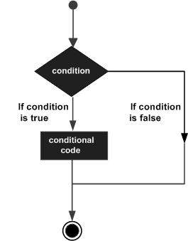
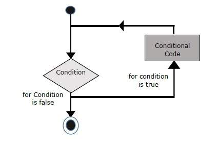
Flow Chart of if-else
The following flow chart shows how the if-else statement works.
JavaScript supports the following forms of if..else statement −
if statement
if…else statement
if…else if… statement.
if statement
The if statement is the fundamental control statement that allows JavaScript to make decisions and execute statements conditionally.
Syntax
The syntax for a basic if statement is as follows −
if (expression) {
   Statement(s) to be executed if expression is true
}
Here a JavaScript expression is evaluated. If the resulting value is true, the given statement(s) are executed. If the expression is false, then no statement would be not executed. Most of the times, you will use comparison operators while making decisions.
Example
Try the following example to understand how the if statement works.
<html><body><script type ="text/javascript"><!--var age =20;if( age >18){
               document.write("<b>Qualifies for driving</b>");}//--></script><p>Set the variable to different value and then try...</p></body></html>
Output
Qualifies for driving
Set the variable to different value and then try...
if…else statement
The ‘if…else’ statement is the next form of control statement that allows JavaScript to execute statements in a more controlled way.
Syntax
if (expression) {
   Statement(s) to be executed if expression is true
} else {
   Statement(s) to be executed if expression is false
}
Here JavaScript expression is evaluated. If the resulting value is true, the given statement(s) in the if block, are executed. If the expression is false, then the given statement(s) in the else block are executed.
Example
Try the following code to learn how to implement an if-else statement in JavaScript.
<html><body><script type ="text/javascript"><!--var age =15;if( age >18){
               document.write("<b>Qualifies for driving</b>");}else{
               document.write("<b>Does not qualify for driving</b>");}//--></script><p>Set the variable to different value and then try...</p></body></html>
Output
Does not qualify for driving
Set the variable to different value and then try...
if…else if… statement
The if…else if… statement is an advanced form of ifelse that allows JavaScript to make a correct decision out of several conditions.
Syntax
The syntax of an if-else-if statement is as follows −
if (expression 1) {
   Statement(s) to be executed if expression 1 is true
} else if (expression 2) {
   Statement(s) to be executed if expression 2 is true
} else if (expression 3) {
   Statement(s) to be executed if expression 3 is true
} else {
   Statement(s) to be executed if no expression is true
}
There is nothing special about this code. It is just a series of if statements, where each if is a part of the else clause of the previous statement. Statement(s) are executed based on the true condition, if none of the conditions is true, then the else block is executed.
Example
Try the following code to learn how to implement an if-else-if statement in JavaScript.
<html><body><script type ="text/javascript"><!--var book ="maths";if( book =="history"){
               document.write("<b>History Book</b>");}elseif( book =="maths"){
               document.write("<b>Maths Book</b>");}elseif( book =="economics"){
               document.write("<b>Economics Book</b>");}else{
               document.write("<b>Unknown Book</b>");}//--></script><p>Set the variable to different value and then try...</p></body><html>
Output
Maths Book
Set the variable to different value and then try...
JavaScript – Switch Case
You can use multiple if…elseif statements, as in the previous chapter, to perform a multiway branch. However, this is not always the best solution, especially when all of the branches depend on the value of a single variable.
Starting with JavaScript 1.2, you can use a switch statement which handles exactly this situation, and it does so more efficiently than repeated if…else if statements.
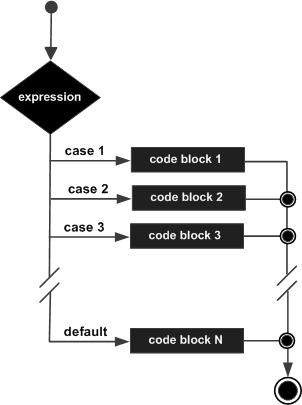
Flow Chart
The following flow chart explains a switch-case statement works.
Syntax
The objective of a switch statement is to give an expression to evaluate and several different statements to execute based on the value of the expression. The interpreter checks each case against the value of the expression until a match is found. If nothing matches, a default condition will be used.
switch (expression) {
   case condition 1: statement(s)
   break;

   case condition 2: statement(s)
   break;
   ...

   case condition n: statement(s)
   break;

   default: statement(s)
}
The break statements indicate the end of a particular case. If they were omitted, the interpreter would continue executing each statement in each of the following cases.
We will explain break statement in Loop Control chapter.
Example
Try the following example to implement switch-case statement.
<html><body><script type ="text/javascript"><!--var grade ='A';
            document.write("Entering switch block<br />");switch(grade){case'A': document.write("Good job<br />");break;case'B': document.write("Pretty good<br />");break;case'C': document.write("Passed<br />");break;case'D': document.write("Not so good<br />");break;case'F': document.write("Failed<br />");break;default:  document.write("Unknown grade<br />")}
            document.write("Exiting switch block");//--></script><p>Set the variable to different value and then try...</p></body></html>
Output
Entering switch block
Good job
Exiting switch block
Set the variable to different value and then try...
Break statements play a major role in switch-case statements. Try the following code that uses switch-case statement without any break statement.
<html><body><script type ="text/javascript"><!--var grade ='A';
            document.write("Entering switch block<br />");switch(grade){case'A': document.write("Good job<br />");case'B': document.write("Pretty good<br />");case'C': document.write("Passed<br />");case'D': document.write("Not so good<br />");case'F': document.write("Failed<br />");default: document.write("Unknown grade<br />")}
            document.write("Exiting switch block");//--></script><p>Set the variable to different value and then try...</p></body></html>
Output
Entering switch block
Good job
Pretty good
Passed
Not so good
Failed
Unknown grade
Exiting switch block
Set the variable to different value and then try...
JavaScript – While Loops
While writing a program, you may encounter a situation where you need to perform an action over and over again. In such situations, you would need to write loop statements to reduce the number of lines.
JavaScript supports all the necessary loops to ease down the pressure of programming.
The while Loop
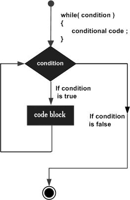
The most basic loop in JavaScript is the while loop which would be discussed in this chapter. The purpose of a while loop is to execute a statement or code block repeatedly as long as an expression is true. Once the expression becomes false, the loop terminates.
Flow Chart
The flow chart of while loop looks as follows −
Syntax
The syntax of while loop in JavaScript is as follows −
while (expression) {
   Statement(s) to be executed if expression is true
}
Example
Try the following example to implement while loop.
<html><body><script type ="text/javascript"><!--var count =0;
            document.write("Starting Loop ");while(count <10){
               document.write("Current Count : "+ count +"<br />");
               count++;}

            document.write("Loop stopped!");//--></script><p>Set the variable to different value and then try...</p></body></html>
Output
Starting Loop
Current Count : 0
Current Count : 1
Current Count : 2
Current Count : 3
Current Count : 4
Current Count : 5
Current Count : 6
Current Count : 7
Current Count : 8
Current Count : 9
Loop stopped!
Set the variable to different value and then try...
The do…while Loop
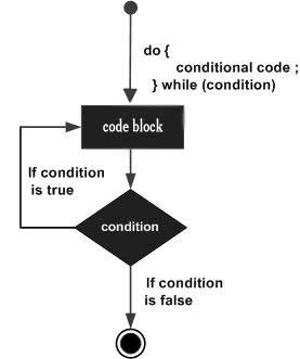
The do…while loop is similar to the while loop except that the condition check happens at the end of the loop. This means that the loop will always be executed at least once, even if the condition is false.
Flow Chart
The flow chart of a do-while loop would be as follows −
Syntax
The syntax for do-while loop in JavaScript is as follows −
do {
   Statement(s) to be executed;
} while (expression);
Note − Dont miss the semicolon used at the end of the do…while loop.
Example
Try the following example to learn how to implement a do-while loop in JavaScript.
<html><body><script type ="text/javascript"><!--var count =0;

            document.write("Starting Loop"+"<br />");do{
               document.write("Current Count : "+ count +"<br />");
               count++;}while(count <5);
            document.write("Loop stopped!");//--></script><p>Set the variable to different value and then try...</p></body></html>
Output
Starting Loop
Current Count : 0
Current Count : 1
Current Count : 2
Current Count : 3
Current Count : 4
Loop Stopped!
Set the variable to different value and then try...
JavaScript – For Loop
The ‘for‘ loop is the most compact form of looping. It includes the following three important parts −
The loop initialization where we initialize our counter to a starting value. The initialization statement is executed before the loop begins.
The test statement which will test if a given condition is true or not. If the condition is true, then the code given inside the loop will be executed, otherwise the control will come out of the loop.
The iteration statement where you can increase or decrease your counter.
You can put all the three parts in a single line separated by semicolons.
Flow Chart
The flow chart of a for loop in JavaScript would be as follows −
Syntax
The syntax of for loop is JavaScript is as follows −
for (initialization; test condition; iteration statement) {
   Statement(s) to be executed if test condition is true
}
Example
Try the following example to learn how a for loop works in JavaScript.
<html><body><script type ="text/javascript"><!--var count;
            document.write("Starting Loop"+"<br />");for(count =0; count <10; count++){
               document.write("Current Count : "+ count );
               document.write("<br />");}
            document.write("Loop stopped!");//--></script><p>Set the variable to different value and then try...</p></body></html>
Output
Starting Loop
Current Count : 0
Current Count : 1
Current Count : 2
Current Count : 3
Current Count : 4
Current Count : 5
Current Count : 6
Current Count : 7
Current Count : 8
Current Count : 9
Loop stopped!
Set the variable to different value and then try...
JavaScript for…in loop
The for…in loop is used to loop through an object’s properties. As we have not discussed Objects yet, you may not feel comfortable with this loop. But once you understand how objects behave in JavaScript, you will find this loop very useful.
Syntax
The syntax of for..in loop is −
for (variablename in object) {
   statement or block to execute
}
In each iteration, one property from object is assigned to variablename and this loop continues till all the properties of the object are exhausted.
Example
Try the following example to implement for-in loop. It prints the web browsers Navigator object.
<html><body><script type ="text/javascript"><!--var aProperty;
            document.write("Navigator Object Properties<br /> ");for(aProperty in navigator){
               document.write(aProperty);
               document.write("<br />");}
            document.write("Exiting from the loop!");//--></script><p>Set the variable to different object and then try...</p></body></html>
Output
Navigator Object Properties
serviceWorker
webkitPersistentStorage
webkitTemporaryStorage
geolocation
doNotTrack
onLine
languages
language
userAgent
product
platform
appVersion
appName
appCodeName
hardwareConcurrency
maxTouchPoints
vendorSub
vendor
productSub
cookieEnabled
mimeTypes
plugins
javaEnabled
getStorageUpdates
getGamepads
webkitGetUserMedia
vibrate
getBattery
sendBeacon
registerProtocolHandler
unregisterProtocolHandler
Exiting from the loop!
Set the variable to different object and then try...
JavaScript – Loop Control
JavaScript provides full control to handle loops and switch statements. There may be a situation when you need to come out of a loop without reaching its bottom. There may also be a situation when you want to skip a part of your code block and start the next iteration of the loop.
To handle all such situations, JavaScript provides break and continue statements. These statements are used to immediately come out of any loop or to start the next iteration of any loop respectively.
The break Statement
The break statement, which was briefly introduced with the switch statement, is used to exit a loop early, breaking out of the enclosing curly braces.
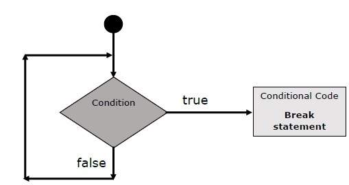
Flow Chart
The flow chart of a break statement would look as follows −
Example
The following example illustrates the use of a break statement with a while loop. Notice how the loop breaks out early once x reaches 5 and reaches to document.write (..) statement just below to the closing curly brace −
<html><body><script type ="text/javascript"><!--var x =1;
         document.write("Entering the loop<br /> ");while(x <20){if(x ==5){break;// breaks out of loop completely}
            x = x +1;
            document.write( x +"<br />");}
         document.write("Exiting the loop!<br /> ");//--></script><p>Set the variable to different value and then try...</p></body></html>
Output
Entering the loop
2
3
4
5
Exiting the loop!
Set the variable to different value and then try...
We already have seen the usage of break statement inside a switch statement.
The continue Statement
The continue statement tells the interpreter to immediately start the next iteration of the loop and skip the remaining code block. When a continue statement is encountered, the program flow moves to the loop check expression immediately and if the condition remains true, then it starts the next iteration, otherwise the control comes out of the loop.
Example
This example illustrates the use of a continue statement with a while loop. Notice how the continue statement is used to skip printing when the index held in variable x reaches 5 −
<html><body><script type ="text/javascript"><!--var x =1;
            document.write("Entering the loop<br /> ");while(x <10){
               x = x +1;if(x ==5){continue;// skip rest of the loop body}
               document.write( x +"<br />");}
            document.write("Exiting the loop!<br /> ");//--></script><p>Set the variable to different value and then try...</p></body></html>
Output
Entering the loop
2
3
4
6
7
8
9
10
Exiting the loop!
Set the variable to different value and then try...
Using Labels to Control the Flow
Starting from JavaScript 1.2, a label can be used with break and continue to control the flow more precisely. A label is simply an identifier followed by a colon (:) that is applied to a statement or a block of code. We will see two different examples to understand how to use labels with break and continue.
Note − Line breaks are not allowed between the continue or break statement and its label name. Also, there should not be any other statement in between a label name and associated loop.
Try the following two examples for a better understanding of Labels.
Example 1
The following example shows how to implement Label with a break statement.
<html><body><script type ="text/javascript"><!--
            document.write("Entering the loop!<br /> ");
            outerloop:// This is the label name         for(var i =0; i <5; i++){
               document.write("Outerloop: "+ i +"<br />");
               innerloop:for(var j =0; j <5; j++){if(j >3)break;// Quit the innermost loopif(i ==2)break innerloop;// Do the same thingif(i ==4)break outerloop;// Quit the outer loop
                  document.write("Innerloop: "+ j +" <br />");}}
            document.write("Exiting the loop!<br /> ");//--></script></body></html>
<html><body><script type ="text/javascript"><!--
         document.write("Entering the loop!<br /> ");
         outerloop:// This is the label namefor(var i =0; i <3; i++){
            document.write("Outerloop: "+ i +"<br />");for(var j =0; j <5; j++){if(j ==3){continue outerloop;}
               document.write("Innerloop: "+ j +"<br />");}}

         document.write("Exiting the loop!<br /> ");//--></script></body></html>
A function is a group of reusable code which can be called anywhere in your program. This eliminates the need of writing the same code again and again. It helps programmers in writing modular codes. Functions allow a programmer to divide a big program into a number of small and manageable functions.
Like any other advanced programming language, JavaScript also supports all the features necessary to write modular code using functions. You must have seen functions like alert() and write() in the earlier chapters. We were using these functions again and again, but they had been written in core JavaScript only once.
JavaScript allows us to write our own functions as well. This section explains how to write your own functions in JavaScript.
Function Definition
Before we use a function, we need to define it. The most common way to define a function in JavaScript is by using the function keyword, followed by a unique function name, a list of parameters (that might be empty), and a statement block surrounded by curly braces.
Syntax
The basic syntax is shown here.
<script type = "text/javascript">
   <!--
      function functionname(parameter-list) {
         statements
      }
   //-->
</script>
Example
Try the following example. It defines a function called sayHello that takes no parameters −
<script type ="text/javascript"><!--functionsayHello(){alert("Hello there");}//--></script>
Calling a Function
To invoke a function somewhere later in the script, you would simply need to write the name of that function as shown in the following code.
<html><head><script type ="text/javascript">functionsayHello(){
            document.write("Hello there!");}</script></head><body><p>Click the following button to call the function</p><form><input type ="button" onclick ="sayHello()" value ="Say Hello"></form><p>Use different text in write method and then try...</p></body></html>
Till now, we have seen functions without parameters. But there is a facility to pass different parameters while calling a function. These passed parameters can be captured inside the function and any manipulation can be done over those parameters. A function can take multiple parameters separated by comma.
Example
Try the following example. We have modified our sayHello function here. Now it takes two parameters.
<html><head><script type ="text/javascript">functionsayHello(name, age){
            document.write(name +" is "+ age +" years old.");}</script></head><body><p>Click the following button to call the function</p><form><input type ="button" onclick ="sayHello('Zara', 7)" value ="Say Hello"></form><p>Use different parameters inside the function and then try...</p></body></html>
A JavaScript function can have an optional return statement. This is required if you want to return a value from a function. This statement should be the last statement in a function.
For example, you can pass two numbers in a function and then you can expect the function to return their multiplication in your calling program.
Example
Try the following example. It defines a function that takes two parameters and concatenates them before returning the resultant in the calling program.
<html><head><script type ="text/javascript">functionconcatenate(first, last){var full;
            full = first + last;return full;}functionsecondFunction(){var result;
            result =concatenate('Zara','Ali');
            document.write(result );}</script></head><body><p>Click the following button to call the function</p><form><input type ="button" onclick ="secondFunction()" value ="Call Function"></form><p>Use different parameters inside the function and then try...</p></body></html>
JavaScript’s interaction with HTML is handled through events that occur when the user or the browser manipulates a page.
When the page loads, it is called an event. When the user clicks a button, that click too is an event. Other examples include events like pressing any key, closing a window, resizing a window, etc.
Developers can use these events to execute JavaScript coded responses, which cause buttons to close windows, messages to be displayed to users, data to be validated, and virtually any other type of response imaginable.
Events are a part of the Document Object Model (DOM) Level 3 and every HTML element contains a set of events which can trigger JavaScript Code.
Please go through this small tutorial for a better understanding HTML Event Reference. Here we will see a few examples to understand a relation between Event and JavaScript −
onclick Event Type
This is the most frequently used event type which occurs when a user clicks the left button of his mouse. You can put your validation, warning etc., against this event type.
Example
Try the following example.
<html><head><script type ="text/javascript"><!--functionsayHello(){alert("Hello World")}//--></script></head><body><p>Click the following button and see result</p><form><input type ="button" onclick ="sayHello()" value ="Say Hello"/></form></body></html>
onsubmit is an event that occurs when you try to submit a form. You can put your form validation against this event type.
Example
The following example shows how to use onsubmit. Here we are calling a validate() function before submitting a form data to the webserver. If validate() function returns true, the form will be submitted, otherwise it will not submit the data.
Try the following example.
<html><head><script type ="text/javascript"><!--functionvalidation(){
               all validation goes here
               .........return either true or false}//--></script></head><body><form method ="POST" action ="t.cgi" onsubmit ="return validate()">.......<input type ="submit" value ="Submit"/></form></body></html>
onmouseover and onmouseout
These two event types will help you create nice effects with images or even with text as well. The onmouseover event triggers when you bring your mouse over any element and the onmouseout triggers when you move your mouse out from that element. Try the following example.
<html><head><script type ="text/javascript"><!--functionover(){
               document.write("Mouse Over");}functionout(){
               document.write("Mouse Out");}//--></script></head><body><p>Bring your mouse inside the division to see the result:</p><div onmouseover ="over()" onmouseout ="out()"><h2> This is inside the division </h2></div></body></html>
The standard HTML 5 events are listed here for your reference. Here script indicates a Javascript function to be executed against that event.
Attribute
Value
Description
Offline
script
Triggers when the document goes offline
Onabort
script
Triggers on an abort event
onafterprint
script
Triggers after the document is printed
onbeforeonload
script
Triggers before the document loads
onbeforeprint
script
Triggers before the document is printed
onblur
script
Triggers when the window loses focus
oncanplay
script
Triggers when media can start play, but might has to stop for buffering
oncanplaythrough
script
Triggers when media can be played to the end, without stopping for buffering
onchange
script
Triggers when an element changes
onclick
script
Triggers on a mouse click
oncontextmenu
script
Triggers when a context menu is triggered
ondblclick
script
Triggers on a mouse double-click
ondrag
script
Triggers when an element is dragged
ondragend
script
Triggers at the end of a drag operation
ondragenter
script
Triggers when an element has been dragged to a valid drop target
ondragleave
script
Triggers when an element is being dragged over a valid drop target
ondragover
script
Triggers at the start of a drag operation
ondragstart
script
Triggers at the start of a drag operation
ondrop
script
Triggers when dragged element is being dropped
ondurationchange
script
Triggers when the length of the media is changed
onemptied
script
Triggers when a media resource element suddenly becomes empty.
onended
script
Triggers when media has reach the end
onerror
script
Triggers when an error occur
onfocus
script
Triggers when the window gets focus
onformchange
script
Triggers when a form changes
onforminput
script
Triggers when a form gets user input
onhaschange
script
Triggers when the document has change
oninput
script
Triggers when an element gets user input
oninvalid
script
Triggers when an element is invalid
onkeydown
script
Triggers when a key is pressed
onkeypress
script
Triggers when a key is pressed and released
onkeyup
script
Triggers when a key is released
onload
script
Triggers when the document loads
onloadeddata
script
Triggers when media data is loaded
onloadedmetadata
script
Triggers when the duration and other media data of a media element is loaded
onloadstart
script
Triggers when the browser starts to load the media data
onmessage
script
Triggers when the message is triggered
onmousedown
script
Triggers when a mouse button is pressed
onmousemove
script
Triggers when the mouse pointer moves
onmouseout
script
Triggers when the mouse pointer moves out of an element
onmouseover
script
Triggers when the mouse pointer moves over an element
onmouseup
script
Triggers when a mouse button is released
onmousewheel
script
Triggers when the mouse wheel is being rotated
onoffline
script
Triggers when the document goes offline
onoine
script
Triggers when the document comes online
ononline
script
Triggers when the document comes online
onpagehide
script
Triggers when the window is hidden
onpageshow
script
Triggers when the window becomes visible
onpause
script
Triggers when media data is paused
onplay
script
Triggers when media data is going to start playing
onplaying
script
Triggers when media data has start playing
onpopstate
script
Triggers when the window’s history changes
onprogress
script
Triggers when the browser is fetching the media data
onratechange
script
Triggers when the media data’s playing rate has changed
onreadystatechange
script
Triggers when the ready-state changes
onredo
script
Triggers when the document performs a redo
onresize
script
Triggers when the window is resized
onscroll
script
Triggers when an element’s scrollbar is being scrolled
onseeked
script
Triggers when a media element’s seeking attribute is no longer true, and the seeking has ended
onseeking
script
Triggers when a media element’s seeking attribute is true, and the seeking has begun
onselect
script
Triggers when an element is selected
onstalled
script
Triggers when there is an error in fetching media data
onstorage
script
Triggers when a document loads
onsubmit
script
Triggers when a form is submitted
onsuspend
script
Triggers when the browser has been fetching media data, but stopped before the entire media file was fetched
ontimeupdate
script
Triggers when media changes its playing position
onundo
script
Triggers when a document performs an undo
onunload
script
Triggers when the user leaves the document
onvolumechange
script
Triggers when media changes the volume, also when volume is set to “mute”
onwaiting
script
Triggers when media has stopped playing, but is expected to resume
JavaScript and Cookies
What are Cookies ?
Web Browsers and Servers use HTTP protocol to communicate and HTTP is a stateless protocol. But for a commercial website, it is required to maintain session information among different pages. For example, one user registration ends after completing many pages. But how to maintain users’ session information across all the web pages.
In many situations, using cookies is the most efficient method of remembering and tracking preferences, purchases, commissions, and other information required for better visitor experience or site statistics.
How It Works ?
Your server sends some data to the visitor’s browser in the form of a cookie. The browser may accept the cookie. If it does, it is stored as a plain text record on the visitor’s hard drive. Now, when the visitor arrives at another page on your site, the browser sends the same cookie to the server for retrieval. Once retrieved, your server knows/remembers what was stored earlier.
Cookies are a plain text data record of 5 variable-length fields −
Expires − The date the cookie will expire. If this is blank, the cookie will expire when the visitor quits the browser.
Domain − The domain name of your site.
Path − The path to the directory or web page that set the cookie. This may be blank if you want to retrieve the cookie from any directory or page.
Secure − If this field contains the word “secure”, then the cookie may only be retrieved with a secure server. If this field is blank, no such restriction exists.
Name=Value − Cookies are set and retrieved in the form of key-value pairs
Cookies were originally designed for CGI programming. The data contained in a cookie is automatically transmitted between the web browser and the web server, so CGI scripts on the server can read and write cookie values that are stored on the client.
JavaScript can also manipulate cookies using the cookie property of the Document object. JavaScript can read, create, modify, and delete the cookies that apply to the current web page.
Storing Cookies
The simplest way to create a cookie is to assign a string value to the document.cookie object, which looks like this.
Here the expires attribute is optional. If you provide this attribute with a valid date or time, then the cookie will expire on a given date or time and thereafter, the cookies’ value will not be accessible.
Note − Cookie values may not include semicolons, commas, or whitespace. For this reason, you may want to use the JavaScript escape() function to encode the value before storing it in the cookie. If you do this, you will also have to use the corresponding unescape() function when you read the cookie value.
Example
Try the following. It sets a customer name in an input cookie.
<html><head><script type ="text/javascript"><!--functionWriteCookie(){if( document.myform.customer.value ==""){alert("Enter some value!");return;}
               cookievalue =escape(document.myform.customer.value)+";";
               document.cookie ="name="+ cookievalue;
               document.write("Setting Cookies : "+"name="+ cookievalue );}//--></script></head><body><form name ="myform" action ="">
         Enter name:<input type ="text" name ="customer"/><input type ="button" value ="Set Cookie" onclick ="WriteCookie();"/></form></body></html>
Now your machine has a cookie called name. You can set multiple cookies using multiple key = value pairs separated by comma.
Reading Cookies
Reading a cookie is just as simple as writing one, because the value of the document.cookie object is the cookie. So you can use this string whenever you want to access the cookie. The document.cookie string will keep a list of name=value pairs separated by semicolons, where name is the name of a cookie and value is its string value.
You can use strings’ split() function to break a string into key and values as follows −
Example
Try the following example to get all the cookies.
<html><head><script type ="text/javascript"><!--functionReadCookie(){var allcookies = document.cookie;
               document.write("All Cookies : "+ allcookies );// Get all the cookies pairs in an array
               cookiearray = allcookies.split(';');// Now take key value pair out of this arrayfor(var i=0; i<cookiearray.length; i++){
                  name = cookiearray[i].split('=')[0];
                  value = cookiearray[i].split('=')[1];
                  document.write("Key is : "+ name +" and Value is : "+ value);}}//--></script></head><body><form name ="myform" action =""><p> click the following button and see the result:</p><input type ="button" value ="Get Cookie" onclick ="ReadCookie()"/></form></body></html>
Note − Here length is a method of Array class which returns the length of an array. We will discuss Arrays in a separate chapter. By that time, please try to digest it.https://www.tutorialspoint.com/javascript/src/reading_cookies.htm
Note − There may be some other cookies already set on your machine. The above code will display all the cookies set on your machine.
Setting Cookies Expiry Date
You can extend the life of a cookie beyond the current browser session by setting an expiration date and saving the expiry date within the cookie. This can be done by setting the expires attribute to a date and time.
Example
Try the following example. It illustrates how to extend the expiry date of a cookie by 1 Month.
<html><head><script type ="text/javascript"><!--functionWriteCookie(){var now =newDate();
               now.setMonth( now.getMonth()+1);
               cookievalue =escape(document.myform.customer.value)+";"

               document.cookie ="name="+ cookievalue;
               document.cookie ="expires="+ now.toUTCString()+";"
               document.write("Setting Cookies : "+"name="+ cookievalue );}//--></script></head><body><form name ="myform" action ="">
         Enter name:<input type ="text" name ="customer"/><input type ="button" value ="Set Cookie" onclick ="WriteCookie()"/></form></body></html>
Sometimes you will want to delete a cookie so that subsequent attempts to read the cookie return nothing. To do this, you just need to set the expiry date to a time in the past.
Example
Try the following example. It illustrates how to delete a cookie by setting its expiry date to one month behind the current date.
<html><head><script type ="text/javascript"><!--functionWriteCookie(){var now =newDate();
               now.setMonth( now.getMonth()-1);
               cookievalue =escape(document.myform.customer.value)+";"

               document.cookie ="name="+ cookievalue;
               document.cookie ="expires="+ now.toUTCString()+";"
               document.write("Setting Cookies : "+"name="+ cookievalue );}//--></script></head><body><form name ="myform" action ="">
         Enter name:<input type ="text" name ="customer"/><input type ="button" value ="Set Cookie" onclick ="WriteCookie()"/></form></body></html>
You might have encountered a situation where you clicked a URL to reach a page X but internally you were directed to another page Y. It happens due to page redirection. This concept is different from JavaScript Page Refresh.
There could be various reasons why you would like to redirect a user from the original page. We are listing down a few of the reasons −
You did not like the name of your domain and you are moving to a new one. In such a scenario, you may want to direct all your visitors to the new site. Here you can maintain your old domain but put a single page with a page redirection such that all your old domain visitors can come to your new domain.
You have built-up various pages based on browser versions or their names or may be based on different countries, then instead of using your server-side page redirection, you can use client-side page redirection to land your users on the appropriate page.
The Search Engines may have already indexed your pages. But while moving to another domain, you would not like to lose your visitors coming through search engines. So you can use client-side page redirection. But keep in mind this should not be done to fool the search engine, it could lead your site to get banned.
How Page Re-direction Works ?
The implementations of Page-Redirection are as follows.
Example 1
It is quite simple to do a page redirect using JavaScript at client side. To redirect your site visitors to a new page, you just need to add a line in your head section as follows.
<html><head><script type ="text/javascript"><!--functionRedirect(){
               window.location ="https://www.tutorialspoint.com";}//--></script></head><body><p>Click the following button, you will be redirected to home page.</p><form><input type ="button" value ="Redirect Me" onclick ="Redirect();"/></form></body></html>
You can show an appropriate message to your site visitors before redirecting them to a new page. This would need a bit time delay to load a new page. The following example shows how to implement the same. Here setTimeout() is a built-in JavaScript function which can be used to execute another function after a given time interval.
<html><head><script type ="text/javascript"><!--functionRedirect(){
               window.location ="https://www.tutorialspoint.com";}
            document.write("You will be redirected to main page in 10 sec.");setTimeout('Redirect()',10000);//--></script></head><body></body></html>
You will be redirected to tutorialspoint.com main page in 10 seconds!
Example 3
The following example shows how to redirect your site visitors onto a different page based on their browsers.
<html><head><script type ="text/javascript"><!--var browsername = navigator.appName;if( browsername =="Netscape"){
               window.location ="http://www.location.com/ns.htm";}elseif( browsername =="Microsoft Internet Explorer"){
               window.location ="http://www.location.com/ie.htm";}else{
               window.location ="http://www.location.com/other.htm";}//--></script></head><body></body></html>
JavaScript – Dialog Boxes
JavaScript supports three important types of dialog boxes. These dialog boxes can be used to raise and alert, or to get confirmation on any input or to have a kind of input from the users. Here we will discuss each dialog box one by one.
Alert Dialog Box
An alert dialog box is mostly used to give a warning message to the users. For example, if one input field requires to enter some text but the user does not provide any input, then as a part of validation, you can use an alert box to give a warning message.
Nonetheless, an alert box can still be used for friendlier messages. Alert box gives only one button “OK” to select and proceed.
Example
<html><head><script type ="text/javascript"><!--functionWarn(){alert("This is a warning message!");
               document.write("This is a warning message!");}//--></script></head><body><p>Click the following button to see the result:</p><form><input type ="button" value ="Click Me" onclick ="Warn();"/></form></body></html>
A confirmation dialog box is mostly used to take user’s consent on any option. It displays a dialog box with two buttons: OK and Cancel.
If the user clicks on the OK button, the window method confirm() will return true. If the user clicks on the Cancel button, then confirm() returns false. You can use a confirmation dialog box as follows.
Example
<html><head><script type ="text/javascript"><!--functiongetConfirmation(){var retVal =confirm("Do you want to continue ?");if( retVal ==true){
                  document.write("User wants to continue!");returntrue;}else{
                  document.write("User does not want to continue!");returnfalse;}}//--></script></head><body><p>Click the following button to see the result:</p><form><input type ="button" value ="Click Me" onclick ="getConfirmation();"/></form></body></html>
The prompt dialog box is very useful when you want to pop-up a text box to get user input. Thus, it enables you to interact with the user. The user needs to fill in the field and then click OK.
This dialog box is displayed using a method called prompt() which takes two parameters: (i) a label which you want to display in the text box and (ii) a default string to display in the text box.
This dialog box has two buttons: OK and Cancel. If the user clicks the OK button, the window method prompt() will return the entered value from the text box. If the user clicks the Cancel button, the window method prompt() returns null.
Example
The following example shows how to use a prompt dialog box −
<html><head><script type ="text/javascript"><!--functiongetValue(){var retVal =prompt("Enter your name : ","your name here");
               document.write("You have entered : "+ retVal);}//--></script></head><body><p>Click the following button to see the result:</p><form><input type ="button" value ="Click Me" onclick ="getValue();"/></form></body></html>
void is an important keyword in JavaScript which can be used as a unary operator that appears before its single operand, which may be of any type. This operator specifies an expression to be evaluated without returning a value.
Syntax
The syntax of void can be either of the following two −
The most common use of this operator is in a client-side javascript: URL, where it allows you to evaluate an expression for its side-effects without the browser displaying the value of the evaluated expression.
Here the expression alert (‘Warning!!!’) is evaluated but it is not loaded back into the current document −
<html><head><script type ="text/javascript"><!--//--></script></head><body><p>Click the following, This won't react at all...</p><a href ="javascript:void(alert('Warning!!!'))">Click me!</a></body></html>
Take a look at the following example. The following link does nothing because the expression “0” has no effect in JavaScript. Here the expression “0” is evaluated, but it is not loaded back into the current document.
<html><head><script type ="text/javascript"><!--//--></script></head><body><p>Click the following, This won't react at all...</p><a href ="javascript:void(0)">Click me!</a></body></html>
Another use of void is to purposely generate the undefined value as follows.
<html><head><script type ="text/javascript"><!--functiongetValue(){var a,b,c;

               a =void( b =5, c =7);
               document.write('a = '+ a +' b = '+ b +' c = '+ c );}//--></script></head><body><p>Click the following to see the result:</p><form><input type ="button" value ="Click Me" onclick ="getValue();"/></form></body></html>
Many times you would like to place a button on your webpage to print the content of that web page via an actual printer. JavaScript helps you to implement this functionality using the print function of window object.
The JavaScript print function window.print() prints the current web page when executed. You can call this function directly using the onclick event as shown in the following example.
Example
Try the following example.
<html><head><script type ="text/javascript"><!--//--></script></head><body><form><input type ="button" value ="Print" onclick ="window.print()"/></form></body><html>
Although it serves the purpose of getting a printout, it is not a recommended way. A printer friendly page is really just a page with text, no images, graphics, or advertising.
You can make a page printer friendly in the following ways −
Make a copy of the page and leave out unwanted text and graphics, then link to that printer friendly page from the original. Check Example.
If you do not want to keep an extra copy of a page, then you can mark your printable text using proper comments like <!– PRINT STARTS HERE –>….. <!– PRINT ENDS HERE –> and then you can use PERL or any other script in the background to purge printable text and display for final printing. We at Tutorialspoint use this method to provide print facility to our site visitors.
How to Print a Page?
If you dont find the above facilities on a web page, then you can use the browser’s standard toolbar to get print the web page. Follow the link as follows.
File → Print → Click OK button.
JavaScript – Objects Overview
JavaScript is an Object Oriented Programming (OOP) language. A programming language can be called object-oriented if it provides four basic capabilities to developers −
Encapsulation − the capability to store related information, whether data or methods, together in an object.
Aggregation − the capability to store one object inside another object.
Inheritance − the capability of a class to rely upon another class (or number of classes) for some of its properties and methods.
Polymorphism − the capability to write one function or method that works in a variety of different ways.
Objects are composed of attributes. If an attribute contains a function, it is considered to be a method of the object, otherwise the attribute is considered a property.
Object Properties
Object properties can be any of the three primitive data types, or any of the abstract data types, such as another object. Object properties are usually variables that are used internally in the object’s methods, but can also be globally visible variables that are used throughout the page.
The syntax for adding a property to an object is −
objectName.objectProperty = propertyValue;
For example − The following code gets the document title using the “title” property of the document object.
var str = document.title;
Object Methods
Methods are the functions that let the object do something or let something be done to it. There is a small difference between a function and a method at a function is a standalone unit of statements and a method is attached to an object and can be referenced by the this keyword.
Methods are useful for everything from displaying the contents of the object to the screen to performing complex mathematical operations on a group of local properties and parameters.
For example − Following is a simple example to show how to use the write() method of document object to write any content on the document.
document.write("This is test");
User-Defined Objects
All user-defined objects and built-in objects are descendants of an object called Object.
The new Operator
The new operator is used to create an instance of an object. To create an object, the new operator is followed by the constructor method.
In the following example, the constructor methods are Object(), Array(), and Date(). These constructors are built-in JavaScript functions.
var employee =newObject();var books =newArray("C++","Perl","Java");var day =newDate("August 15, 1947");
The Object() Constructor
A constructor is a function that creates and initializes an object. JavaScript provides a special constructor function called Object() to build the object. The return value of the Object() constructor is assigned to a variable.
The variable contains a reference to the new object. The properties assigned to the object are not variables and are not defined with the var keyword.
Example 1
Try the following example; it demonstrates how to create an Object.
<html><head><title>User-defined objects</title><script type ="text/javascript">var book =newObject();// Create the object
         book.subject ="Perl";// Assign properties to the object
         book.author  ="Mohtashim";</script></head><body><script type ="text/javascript">
         document.write("Book name is : "+ book.subject +"<br>");
         document.write("Book author is : "+ book.author +"<br>");</script></body></html>
Output
Book name is : Perl
Book author is : Mohtashim
Example 2
This example demonstrates how to create an object with a User-Defined Function. Here this keyword is used to refer to the object that has been passed to a function.
<html><head><title>User-defined objects</title><script type ="text/javascript">functionbook(title, author){this.title = title;this.author  = author;}</script></head><body><script type ="text/javascript">var myBook =newbook("Perl","Mohtashim");
         document.write("Book title is : "+ myBook.title +"<br>");
         document.write("Book author is : "+ myBook.author +"<br>");</script></body></html>
Output
Book title is : Perl
Book author is : Mohtashim
Defining Methods for an Object
The previous examples demonstrate how the constructor creates the object and assigns properties. But we need to complete the definition of an object by assigning methods to it.
Example
Try the following example; it shows how to add a function along with an object.
<html><head><title>User-defined objects</title><script type ="text/javascript">// Define a function which will work as a methodfunctionaddPrice(amount){this.price = amount;}functionbook(title, author){this.title = title;this.author  = author;this.addPrice = addPrice;// Assign that method as property.}</script></head><body><script type ="text/javascript">var myBook =newbook("Perl","Mohtashim");
         myBook.addPrice(100);

         document.write("Book title is : "+ myBook.title +"<br>");
         document.write("Book author is : "+ myBook.author +"<br>");
         document.write("Book price is : "+ myBook.price +"<br>");</script></body></html>
Output
Book title is : Perl
Book author is : Mohtashim
Book price is : 100
The ‘with’ Keyword
The with keyword is used as a kind of shorthand for referencing an object’s properties or methods.
The object specified as an argument to with becomes the default object for the duration of the block that follows. The properties and methods for the object can be used without naming the object.
Syntax
The syntax for with object is as follows −
with (object) {
   properties used without the object name and dot
}
Example
Try the following example.
<html><head><title>User-defined objects</title><script type ="text/javascript">// Define a function which will work as a methodfunctionaddPrice(amount){with(this){
               price = amount;}}functionbook(title, author){this.title = title;this.author = author;this.price =0;this.addPrice = addPrice;// Assign that method as property.}</script></head><body><script type ="text/javascript">var myBook =newbook("Perl","Mohtashim");
         myBook.addPrice(100);

         document.write("Book title is : "+ myBook.title +"<br>");
         document.write("Book author is : "+ myBook.author +"<br>");
         document.write("Book price is : "+ myBook.price +"<br>");</script></body></html>
Output
Book title is : Perl
Book author is : Mohtashim
Book price is : 100
JavaScript Native Objects
JavaScript has several built-in or native objects. These objects are accessible anywhere in your program and will work the same way in any browser running in any operating system.
Here is the list of all important JavaScript Native Objects −
The Number object represents numerical date, either integers or floating-point numbers. In general, you do not need to worry about Number objects because the browser automatically converts number literals to instances of the number class.
Syntax
The syntax for creating a number object is as follows −
var val = new Number(number);
In the place of number, if you provide any non-number argument, then the argument cannot be converted into a number, it returns NaN (Not-a-Number).
Number Properties
Here is a list of each property and their description.
Sr.No.
Property & Description
1
MAX_VALUEThe largest possible value a number in JavaScript can have 1.7976931348623157E+308
2
MIN_VALUEThe smallest possible value a number in JavaScript can have 5E-324
prototypeA static property of the Number object. Use the prototype property to assign new properties and methods to the Number object in the current document
7
constructorReturns the function that created this object’s instance. By default this is the Number object.
In the following sections, we will take a few examples to demonstrate the properties of Number.
Number Methods
The Number object contains only the default methods that are a part of every object’s definition.
Sr.No.
Method & Description
1
toExponential()Forces a number to display in exponential notation, even if the number is in the range in which JavaScript normally uses standard notation.
2
toFixed()Formats a number with a specific number of digits to the right of the decimal.
3
toLocaleString()Returns a string value version of the current number in a format that may vary according to a browser’s local settings.
4
toPrecision()Defines how many total digits (including digits to the left and right of the decimal) to display of a number.
5
toString()Returns the string representation of the number’s value.
In the following sections, we will have a few examples to explain the methods of Number.
JavaScript – The Boolean Object
The Boolean object represents two values, either “true” or “false”. If value parameter is omitted or is 0, -0, null, false, NaN, undefined, or the empty string (“”), the object has an initial value of false.
Syntax
Use the following syntax to create a boolean object.
var val = new Boolean(value);
Boolean Properties
Here is a list of the properties of Boolean object −
Sr.No.
Property & Description
1
constructorReturns a reference to the Boolean function that created the object.
2
prototypeThe prototype property allows you to add properties and methods to an object.
In the following sections, we will have a few examples to illustrate the properties of Boolean object.
Boolean Methods
Here is a list of the methods of Boolean object and their description.
Sr.No.
Method & Description
1
toSource()Returns a string containing the source of the Boolean object; you can use this string to create an equivalent object.
2
toString()Returns a string of either “true” or “false” depending upon the value of the object.
3
valueOf()Returns the primitive value of the Boolean object.
In the following sections, we will have a few examples to demonstrate the usage of the Boolean methods.
JavaScript – The Strings Object
The String object lets you work with a series of characters; it wraps Javascript’s string primitive data type with a number of helper methods.
As JavaScript automatically converts between string primitives and String objects, you can call any of the helper methods of the String object on a string primitive.
Syntax
Use the following syntax to create a String object −
var val = new String(string);
The String parameter is a series of characters that has been properly encoded.
String Properties
Here is a list of the properties of String object and their description.
Sr.No.
Property & Description
1
constructorReturns a reference to the String function that created the object.
prototypeThe prototype property allows you to add properties and methods to an object.
In the following sections, we will have a few examples to demonstrate the usage of String properties.
String Methods
Here is a list of the methods available in String object along with their description.
Sr.No.
Method & Description
1
charAt()Returns the character at the specified index.
2
charCodeAt()Returns a number indicating the Unicode value of the character at the given index.
3
concat()Combines the text of two strings and returns a new string.
4
indexOf()Returns the index within the calling String object of the first occurrence of the specified value, or -1 if not found.
5
lastIndexOf()Returns the index within the calling String object of the last occurrence of the specified value, or -1 if not found.
6
localeCompare()Returns a number indicating whether a reference string comes before or after or is the same as the given string in sort order.
7
match()Used to match a regular expression against a string.
8
replace()Used to find a match between a regular expression and a string, and to replace the matched substring with a new substring.
9
search()Executes the search for a match between a regular expression and a specified string.
10
slice()Extracts a section of a string and returns a new string.
11
split()Splits a String object into an array of strings by separating the string into substrings.
12
substr()Returns the characters in a string beginning at the specified location through the specified number of characters.
13
substring()Returns the characters in a string between two indexes into the string.
14
toLocaleLowerCase()The characters within a string are converted to lower case while respecting the current locale.
15
toLocaleUpperCase()The characters within a string are converted to upper case while respecting the current locale.
16
toLowerCase()Returns the calling string value converted to lower case.
17
toString()Returns a string representing the specified object.
18
toUpperCase()Returns the calling string value converted to uppercase.
19
valueOf()Returns the primitive value of the specified object.
String HTML Wrappers
Here is a list of the methods that return a copy of the string wrapped inside an appropriate HTML tag.
Sr.No.
Method & Description
1
anchor()Creates an HTML anchor that is used as a hypertext target.
2
big()Creates a string to be displayed in a big font as if it were in a <big> tag.
3
blink()Creates a string to blink as if it were in a <blink> tag.
4
bold()Creates a string to be displayed as bold as if it were in a <b> tag.
5
fixed()Causes a string to be displayed in fixed-pitch font as if it were in a <tt> tag
6
fontcolor()Causes a string to be displayed in the specified color as if it were in a <font color=”color”> tag.
7
fontsize()Causes a string to be displayed in the specified font size as if it were in a <font size=”size”> tag.
8
italics()Causes a string to be italic, as if it were in an <i> tag.
9
link()Creates an HTML hypertext link that requests another URL.
10
small()Causes a string to be displayed in a small font, as if it were in a <small> tag.
11
strike()Causes a string to be displayed as struck-out text, as if it were in a <strike> tag.
12
sub()Causes a string to be displayed as a subscript, as if it were in a <sub> tag
13
sup()Causes a string to be displayed as a superscript, as if it were in a <sup> tag
In the following sections, we will have a few examples to demonstrate the usage of String methods.
JavaScript – The Arrays Object
The Array object lets you store multiple values in a single variable. It stores a fixed-size sequential collection of elements of the same type. An array is used to store a collection of data, but it is often more useful to think of an array as a collection of variables of the same type.
Syntax
Use the following syntax to create an Array object −
var fruits = new Array( "apple", "orange", "mango" );
The Array parameter is a list of strings or integers. When you specify a single numeric parameter with the Array constructor, you specify the initial length of the array. The maximum length allowed for an array is 4,294,967,295.
You can create array by simply assigning values as follows −
var fruits =["apple","orange","mango"];
You will use ordinal numbers to access and to set values inside an array as follows.
fruits[0] is the first element
fruits[1] is the second element
fruits[2] is the third element
Array Properties
Here is a list of the properties of the Array object along with their description.
Sr.No.
Property & Description
1
constructorReturns a reference to the array function that created the object.
2
indexThe property represents the zero-based index of the match in the string
3
inputThis property is only present in arrays created by regular expression matches.
4
lengthReflects the number of elements in an array.
5
prototypeThe prototype property allows you to add properties and methods to an object.
In the following sections, we will have a few examples to illustrate the usage of Array properties.
Array Methods
Here is a list of the methods of the Array object along with their description.
Sr.No.
Method & Description
1
concat()Returns a new array comprised of this array joined with other array(s) and/or value(s).
2
every()Returns true if every element in this array satisfies the provided testing function.
3
filter()Creates a new array with all of the elements of this array for which the provided filtering function returns true.
4
forEach()Calls a function for each element in the array.
5
indexOf()Returns the first (least) index of an element within the array equal to the specified value, or -1 if none is found.
6
join()Joins all elements of an array into a string.
7
lastIndexOf()Returns the last (greatest) index of an element within the array equal to the specified value, or -1 if none is found.
8
map()Creates a new array with the results of calling a provided function on every element in this array.
9
pop()Removes the last element from an array and returns that element.
10
push()Adds one or more elements to the end of an array and returns the new length of the array.
11
reduce()Apply a function simultaneously against two values of the array (from left-to-right) as to reduce it to a single value.
12
reduceRight()Apply a function simultaneously against two values of the array (from right-to-left) as to reduce it to a single value.
13
reverse()Reverses the order of the elements of an array — the first becomes the last, and the last becomes the first.
14
shift()Removes the first element from an array and returns that element.
15
slice()Extracts a section of an array and returns a new array.
16
some()Returns true if at least one element in this array satisfies the provided testing function.
splice()Adds and/or removes elements from an array.
20
toString()Returns a string representing the array and its elements.
21
unshift()Adds one or more elements to the front of an array and returns the new length of the array.
In the following sections, we will have a few examples to demonstrate the usage of Array methods.
JavaScript – The Date Object
The Date object is a datatype built into the JavaScript language. Date objects are created with the new Date( ) as shown below.
Once a Date object is created, a number of methods allow you to operate on it. Most methods simply allow you to get and set the year, month, day, hour, minute, second, and millisecond fields of the object, using either local time or UTC (universal, or GMT) time.
The ECMAScript standard requires the Date object to be able to represent any date and time, to millisecond precision, within 100 million days before or after 1/1/1970. This is a range of plus or minus 273,785 years, so JavaScript can represent date and time till the year 275755.
Syntax
You can use any of the following syntaxes to create a Date object using Date() constructor.
new Date( )
new Date(milliseconds)
new Date(datestring)
new Date(year,month,date[,hour,minute,second,millisecond ])
Note − Parameters in the brackets are always optional.
Here is a description of the parameters −
No Argument − With no arguments, the Date() constructor creates a Date object set to the current date and time.
milliseconds − When one numeric argument is passed, it is taken as the internal numeric representation of the date in milliseconds, as returned by the getTime() method. For example, passing the argument 5000 creates a date that represents five seconds past midnight on 1/1/70.
datestring − When one string argument is passed, it is a string representation of a date, in the format accepted by the Date.parse() method.
7 agruments − To use the last form of the constructor shown above. Here is a description of each argument −
year − Integer value representing the year. For compatibility (in order to avoid the Y2K problem), you should always specify the year in full; use 1998, rather than 98.
month − Integer value representing the month, beginning with 0 for January to 11 for December.
date − Integer value representing the day of the month.
hour − Integer value representing the hour of the day (24-hour scale).
minute − Integer value representing the minute segment of a time reading.
second − Integer value representing the second segment of a time reading.
millisecond − Integer value representing the millisecond segment of a time reading.
Date Properties
Here is a list of the properties of the Date object along with their description.
Sr.No.
Property & Description
1
constructorSpecifies the function that creates an object’s prototype.
2
prototypeThe prototype property allows you to add properties and methods to an object
In the following sections, we will have a few examples to demonstrate the usage of different Date properties.
Date Methods
Here is a list of the methods used with Date and their description.
getDate()Returns the day of the month for the specified date according to local time.
3
getDay()Returns the day of the week for the specified date according to local time.
4
getFullYear()Returns the year of the specified date according to local time.
5
getHours()Returns the hour in the specified date according to local time.
6
getMilliseconds()Returns the milliseconds in the specified date according to local time.
7
getMinutes()Returns the minutes in the specified date according to local time.
8
getMonth()Returns the month in the specified date according to local time.
9
getSeconds()Returns the seconds in the specified date according to local time.
10
getTime()Returns the numeric value of the specified date as the number of milliseconds since January 1, 1970, 00:00:00 UTC.
11
getTimezoneOffset()Returns the time-zone offset in minutes for the current locale.
12
getUTCDate()Returns the day (date) of the month in the specified date according to universal time.
13
getUTCDay()Returns the day of the week in the specified date according to universal time.
14
getUTCFullYear()Returns the year in the specified date according to universal time.
15
getUTCHours()Returns the hours in the specified date according to universal time.
16
getUTCMilliseconds()Returns the milliseconds in the specified date according to universal time.
17
getUTCMinutes()Returns the minutes in the specified date according to universal time.
18
getUTCMonth()Returns the month in the specified date according to universal time.
19
getUTCSeconds()Returns the seconds in the specified date according to universal time.
20
getYear()Deprecated – Returns the year in the specified date according to local time. Use getFullYear instead.
21
setDate()Sets the day of the month for a specified date according to local time.
22
setFullYear()Sets the full year for a specified date according to local time.
23
setHours()Sets the hours for a specified date according to local time.
24
setMilliseconds()Sets the milliseconds for a specified date according to local time.
25
setMinutes()Sets the minutes for a specified date according to local time.
26
setMonth()Sets the month for a specified date according to local time.
27
setSeconds()Sets the seconds for a specified date according to local time.
28
setTime()Sets the Date object to the time represented by a number of milliseconds since January 1, 1970, 00:00:00 UTC.
29
setUTCDate()Sets the day of the month for a specified date according to universal time.
30
setUTCFullYear()Sets the full year for a specified date according to universal time.
31
setUTCHours()Sets the hour for a specified date according to universal time.
32
setUTCMilliseconds()Sets the milliseconds for a specified date according to universal time.
33
setUTCMinutes()Sets the minutes for a specified date according to universal time.
34
setUTCMonth()Sets the month for a specified date according to universal time.
35
setUTCSeconds()Sets the seconds for a specified date according to universal time.
36
setYear()Deprecated – Sets the year for a specified date according to local time. Use setFullYear instead.
37
toDateString()Returns the “date” portion of the Date as a human-readable string.
38
toGMTString()Deprecated – Converts a date to a string, using the Internet GMT conventions. Use toUTCString instead.
39
toLocaleDateString()Returns the “date” portion of the Date as a string, using the current locale’s conventions.
40
toLocaleFormat()Converts a date to a string, using a format string.
41
toLocaleString()Converts a date to a string, using the current locale’s conventions.
42
toLocaleTimeString()Returns the “time” portion of the Date as a string, using the current locale’s conventions.
43
toSource()Returns a string representing the source for an equivalent Date object; you can use this value to create a new object.
44
toString()Returns a string representing the specified Date object.
45
toTimeString()Returns the “time” portion of the Date as a human-readable string.
46
toUTCString()Converts a date to a string, using the universal time convention.
47
valueOf()Returns the primitive value of a Date object.
Converts a date to a string, using the universal time convention.
Date Static Methods
In addition to the many instance methods listed previously, the Date object also defines two static methods. These methods are invoked through the Date() constructor itself.
Sr.No.
Method & Description
1
Date.parse( )Parses a string representation of a date and time and returns the internal millisecond representation of that date.
2
Date.UTC( )Returns the millisecond representation of the specified UTC date and time.
In the following sections, we will have a few examples to demonstrate the usages of Date Static methods.
JavaScript – The Math Object
The math object provides you properties and methods for mathematical constants and functions. Unlike other global objects, Math is not a constructor. All the properties and methods of Math are static and can be called by using Math as an object without creating it.
Thus, you refer to the constant pi as Math.PI and you call the sine function as Math.sin(x), where x is the method’s argument.
Syntax
The syntax to call the properties and methods of Math are as follows
var pi_val = Math.PI;
var sine_val = Math.sin(30);
Math Properties
Here is a list of all the properties of Math and their description.
Sr.No.
Property & Description
1
E \Euler’s constant and the base of natural logarithms, approximately 2.718.
In the following sections, we will have a few examples to demonstrate the usage of the methods associated with Math.
Regular Expressions and RegExp Object
A regular expression is an object that describes a pattern of characters.
The JavaScript RegExp class represents regular expressions, and both String and RegExp define methods that use regular expressions to perform powerful pattern-matching and search-and-replace functions on text.
Syntax
A regular expression could be defined with the RegExp () constructor, as follows −
var pattern = new RegExp(pattern, attributes);
or simply
var pattern = /pattern/attributes;
Here is the description of the parameters −
pattern − A string that specifies the pattern of the regular expression or another regular expression.
attributes − An optional string containing any of the “g”, “i”, and “m” attributes that specify global, case-insensitive, and multi-line matches, respectively.
Brackets
Brackets ([]) have a special meaning when used in the context of regular expressions. They are used to find a range of characters.
Sr.No.
Expression & Description
1
[…]Any one character between the brackets.
2
[^…]Any one character not between the brackets.
3
[0-9]It matches any decimal digit from 0 through 9.
4
[a-z]It matches any character from lowercase a through lowercase z.
5
[A-Z]It matches any character from uppercase A through uppercase Z.
6
[a-Z]It matches any character from lowercase a through uppercase Z.
The ranges shown above are general; you could also use the range [0-3] to match any decimal digit ranging from 0 through 3, or the range [b-v] to match any lowercase character ranging from b through v.
Quantifiers
The frequency or position of bracketed character sequences and single characters can be denoted by a special character. Each special character has a specific connotation. The +, *, ?, and $ flags all follow a character sequence.
Sr.No.
Expression & Description
1
p+It matches any string containing one or more p’s.
2
p*It matches any string containing zero or more p’s.
3
p?It matches any string containing at most one p.
4
p{N}It matches any string containing a sequence of N p’s
5
p{2,3}It matches any string containing a sequence of two or three p’s.
6
p{2, }It matches any string containing a sequence of at least two p’s.
7
p$It matches any string with p at the end of it.
8
^pIt matches any string with p at the beginning of it.
Examples
Following examples explain more about matching characters.
Sr.No.
Expression & Description
1
[^a-zA-Z]It matches any string not containing any of the characters ranging from a through z and A through Z.
2
p.pIt matches any string containing p, followed by any character, in turn followed by another p.
3
^.{2}$It matches any string containing exactly two characters.
4
<b>(.*)</b>It matches any string enclosed within <b> and </b>.
5
p(hp)*It matches any string containing a p followed by zero or more instances of the sequence hp.
Literal characters
Sr.No.
Character & Description
1
AlphanumericItself
2
\0The NUL character (\u0000)
3
\tTab (\u0009
4
\nNewline (\u000A)
5
\vVertical tab (\u000B)
6
\fForm feed (\u000C)
7
\rCarriage return (\u000D)
8
\xnnThe Latin character specified by the hexadecimal number nn; for example, \x0A is the same as \n
9
\uxxxxThe Unicode character specified by the hexadecimal number xxxx; for example, \u0009 is the same as \t
10
\cXThe control character ^X; for example, \cJ is equivalent to the newline character \n
Metacharacters
A metacharacter is simply an alphabetical character preceded by a backslash that acts to give the combination a special meaning.
For instance, you can search for a large sum of money using the ‘\d’ metacharacter: /([\d]+)000/, Here \d will search for any string of numerical character.
The following table lists a set of metacharacters which can be used in PERL Style Regular Expressions.
Sr.No.
Character & Description
1
.a single character
2
\sa whitespace character (space, tab, newline)
3
\Snon-whitespace character
4
\da digit (0-9)
5
\Da non-digit
6
\wa word character (a-z, A-Z, 0-9, _)
7
\Wa non-word character
8
[\b]a literal backspace (special case).
9
[aeiou]matches a single character in the given set
10
[^aeiou]matches a single character outside the given set
11
(foo|bar|baz)matches any of the alternatives specified
Modifiers
Several modifiers are available that can simplify the way you work with regexps, like case sensitivity, searching in multiple lines, etc.
Sr.No.
Modifier & Description
1
iPerform case-insensitive matching.
2
mSpecifies that if the string has newline or carriage return characters, the ^ and $ operators will now match against a newline boundary, instead of a string boundary
3
gPerforms a global matchthat is, find all matches rather than stopping after the first match.
RegExp Properties
Here is a list of the properties associated with RegExp and their description.
Sr.No.
Property & Description
1
constructorSpecifies the function that creates an object’s prototype.
toSource()Returns an object literal representing the specified object; you can use this value to create a new object.
4
toString()Returns a string representing the specified object.
In the following sections, we will have a few examples to demonstrate the usage of RegExp methods.
JavaScript – Document Object Model or DOM
Every web page resides inside a browser window which can be considered as an object.
A Document object represents the HTML document that is displayed in that window. The Document object has various properties that refer to other objects which allow access to and modification of document content.
The way a document content is accessed and modified is called the Document Object Model, or DOM. The Objects are organized in a hierarchy. This hierarchical structure applies to the organization of objects in a Web document.
Window object − Top of the hierarchy. It is the outmost element of the object hierarchy.
Document object − Each HTML document that gets loaded into a window becomes a document object. The document contains the contents of the page.
Form object − Everything enclosed in the <form>…</form> tags sets the form object.
Form control elements − The form object contains all the elements defined for that object such as text fields, buttons, radio buttons, and checkboxes.
Here is a simple hierarchy of a few important objects −
There are several DOMs in existence. The following sections explain each of these DOMs in detail and describe how you can use them to access and modify document content.
The Legacy DOM − This is the model which was introduced in early versions of JavaScript language. It is well supported by all browsers, but allows access only to certain key portions of documents, such as forms, form elements, and images.
The W3C DOM − This document object model allows access and modification of all document content and is standardized by the World Wide Web Consortium (W3C). This model is supported by almost all the modern browsers.
The IE4 DOM − This document object model was introduced in Version 4 of Microsoft’s Internet Explorer browser. IE 5 and later versions include support for most basic W3C DOM features.
DOM compatibility
If you want to write a script with the flexibility to use either W3C DOM or IE 4 DOM depending on their availability, then you can use a capability-testing approach that first checks for the existence of a method or property to determine whether the browser has the capability you desire. For example −
if (document.getElementById) {
   // If the W3C method exists, use it
} else if (document.all) {
   // If the all[] array exists, use it
} else {
   // Otherwise use the legacy DOM
}
JavaScript – Errors & Exceptions Handling
There are three types of errors in programming: (a) Syntax Errors, (b) Runtime Errors, and (c) Logical Errors.
Syntax Errors
Syntax errors, also called parsing errors, occur at compile time in traditional programming languages and at interpret time in JavaScript.
For example, the following line causes a syntax error because it is missing a closing parenthesis.
<script type = "text/javascript">
   <!--
      window.print(;
   //-->
</script>
When a syntax error occurs in JavaScript, only the code contained within the same thread as the syntax error is affected and the rest of the code in other threads gets executed assuming nothing in them depends on the code containing the error.
Runtime Errors
Runtime errors, also called exceptions, occur during execution (after compilation/interpretation).
For example, the following line causes a runtime error because here the syntax is correct, but at runtime, it is trying to call a method that does not exist.
<script type = "text/javascript">
   <!--
      window.printme();
   //-->
</script>
Exceptions also affect the thread in which they occur, allowing other JavaScript threads to continue normal execution.
Logical Errors
Logic errors can be the most difficult type of errors to track down. These errors are not the result of a syntax or runtime error. Instead, they occur when you make a mistake in the logic that drives your script and you do not get the result you expected.
You cannot catch those errors, because it depends on your business requirement what type of logic you want to put in your program.
The try…catch…finally Statement
The latest versions of JavaScript added exception handling capabilities. JavaScript implements the try…catch…finally construct as well as the throw operator to handle exceptions.
You can catch programmer-generated and runtime exceptions, but you cannot catch JavaScript syntax errors.
Here is the try…catch…finally block syntax −
<script type ="text/javascript"><!--try{// Code to run[break;]}catch( e ){// Code to run if an exception occurs[break;]}[finally{// Code that is always executed regardless of // an exception occurring}]//--></script>
The try block must be followed by either exactly one catch block or one finally block (or one of both). When an exception occurs in the try block, the exception is placed in e and the catch block is executed. The optional finally block executes unconditionally after try/catch.
Examples
Here is an example where we are trying to call a non-existing function which in turn is raising an exception. Let us see how it behaves without try…catch−
<html><head><script type ="text/javascript"><!--functionmyFunc(){var a =100;alert("Value of variable a is : "+ a );}//--></script></head><body><p>Click the following to see the result:</p><form><input type ="button" value ="Click Me" onclick ="myFunc();"/></form></body></html>
Now let us try to catch this exception using try…catch and display a user-friendly message. You can also suppress this message, if you want to hide this error from a user.
<html><head><script type ="text/javascript"><!--functionmyFunc(){var a =100;try{alert("Value of variable a is : "+ a );}catch( e ){alert("Error: "+ e.description );}}//--></script></head><body><p>Click the following to see the result:</p><form><input type ="button" value ="Click Me" onclick ="myFunc();"/></form></body></html>
You can use finally block which will always execute unconditionally after the try/catch. Here is an example.
<html><head><script type ="text/javascript"><!--functionmyFunc(){var a =100;try{alert("Value of variable a is : "+ a );}catch( e ){alert("Error: "+ e.description );}finally{alert("Finally block will always execute!");}}//--></script></head><body><p>Click the following to see the result:</p><form><input type ="button" value ="Click Me" onclick ="myFunc();"/></form></body></html>
You can use throw statement to raise your built-in exceptions or your customized exceptions. Later these exceptions can be captured and you can take an appropriate action.
Example
The following example demonstrates how to use a throw statement.
<html><head><script type ="text/javascript"><!--functionmyFunc(){var a =100;var b =0;try{if( b ==0){throw("Divide by zero error.");}else{var c = a / b;}}catch( e ){alert("Error: "+ e );}}//--></script></head><body><p>Click the following to see the result:</p><form><input type ="button" value ="Click Me" onclick ="myFunc();"/></form></body></html>
You can raise an exception in one function using a string, integer, Boolean, or an object and then you can capture that exception either in the same function as we did above, or in another function using a try…catch block.
The onerror() Method
The onerror event handler was the first feature to facilitate error handling in JavaScript. The error event is fired on the window object whenever an exception occurs on the page.
<html><head><script type ="text/javascript"><!--
            window.onerror=function(){alert("An error occurred.");}//--></script></head><body><p>Click the following to see the result:</p><form><input type ="button" value ="Click Me" onclick ="myFunc();"/></form></body></html>
The onerror event handler provides three pieces of information to identify the exact nature of the error −
Error message − The same message that the browser would display for the given error
URL − The file in which the error occurred
Line number− The line number in the given URL that caused the error
Here is the example to show how to extract this information.
Example
<html><head><script type ="text/javascript"><!--
            window.onerror=function(msg, url, line){alert("Message : "+ msg );alert("url : "+ url );alert("Line number : "+ line );}//--></script></head><body><p>Click the following to see the result:</p><form><input type ="button" value ="Click Me" onclick ="myFunc();"/></form></body></html>
You can display extracted information in whatever way you think it is better.
You can use an onerror method, as shown below, to display an error message in case there is any problem in loading an image.
<img src="myimage.gif" onerror="alert('An error occurred loading the image.')"/>
You can use onerror with many HTML tags to display appropriate messages in case of errors.
JavaScript – Form Validation
Form validation normally used to occur at the server, after the client had entered all the necessary data and then pressed the Submit button. If the data entered by a client was incorrect or was simply missing, the server would have to send all the data back to the client and request that the form be resubmitted with correct information. This was really a lengthy process which used to put a lot of burden on the server.
JavaScript provides a way to validate form’s data on the client’s computer before sending it to the web server. Form validation generally performs two functions.
Basic Validation − First of all, the form must be checked to make sure all the mandatory fields are filled in. It would require just a loop through each field in the form and check for data.
Data Format Validation − Secondly, the data that is entered must be checked for correct form and value. Your code must include appropriate logic to test correctness of data.
Example
We will take an example to understand the process of validation. Here is a simple form in html format.
<html><head><title>Form Validation</title><script type ="text/javascript"><!--// Form validation code will come here.//--></script></head><body><form action ="/cgi-bin/test.cgi" name ="myForm" onsubmit ="return(validate());"><table cellspacing ="2" cellpadding ="2" border ="1"><tr><td align ="right">Name</td><td><input type ="text" name ="Name"/></td></tr><tr><td align ="right">EMail</td><td><input type ="text" name ="EMail"/></td></tr><tr><td align ="right">Zip Code</td><td><input type ="text" name ="Zip"/></td></tr><tr><td align ="right">Country</td><td><select name ="Country"><option value ="-1" selected>[choose yours]</option><option value ="1">USA</option><option value ="2">UK</option><option value ="3">INDIA</option></select></td></tr><tr><td align ="right"></td><td><input type ="submit" value ="Submit"/></td></tr></table></form></body></html>
First let us see how to do a basic form validation. In the above form, we are calling validate() to validate data when onsubmit event is occurring. The following code shows the implementation of this validate() function.
<script type ="text/javascript"><!--// Form validation code will come here.functionvalidate(){if( document.myForm.Name.value ==""){alert("Please provide your name!");
            document.myForm.Name.focus();returnfalse;}if( document.myForm.EMail.value ==""){alert("Please provide your Email!");
            document.myForm.EMail.focus();returnfalse;}if( document.myForm.Zip.value ==""||isNaN( document.myForm.Zip.value )||
            document.myForm.Zip.value.length !=5){alert("Please provide a zip in the format #####.");
            document.myForm.Zip.focus();returnfalse;}if( document.myForm.Country.value =="-1"){alert("Please provide your country!");returnfalse;}return(true);}//--></script>
Data Format Validation
Now we will see how we can validate our entered form data before submitting it to the web server.
The following example shows how to validate an entered email address. An email address must contain at least a @ sign and a dot (.). Also, the @ must not be the first character of the email address, and the last dot must at least be one character after the @ sign.
You can use JavaScript to create a complex animation having, but not limited to, the following elements −
Fireworks
Fade Effect
Roll-in or Roll-out
Page-in or Page-out
Object movements
You might be interested in existing JavaScript based animation library: Script.Aculo.us.
This tutorial provides a basic understanding of how to use JavaScript to create an animation.
JavaScript can be used to move a number of DOM elements (<img />, <div> or any other HTML element) around the page according to some sort of pattern determined by a logical equation or function.
JavaScript provides the following two functions to be frequently used in animation programs.
setTimeout( function, duration) − This function calls function after duration milliseconds from now.
setInterval(function, duration) − This function calls function after every duration milliseconds.
clearTimeout(setTimeout_variable) − This function calls clears any timer set by the setTimeout() functions.
JavaScript can also set a number of attributes of a DOM object including its position on the screen. You can set top and left attribute of an object to position it anywhere on the screen. Here is its syntax.
// Set distance from left edge of the screen.
object.style.left = distance in pixels or points;

or

// Set distance from top edge of the screen.
object.style.top = distance in pixels or points;
Manual Animation
So let’s implement one simple animation using DOM object properties and JavaScript functions as follows. The following list contains different DOM methods.
We are using the JavaScript function getElementById() to get a DOM object and then assigning it to a global variable imgObj.
We have defined an initialization function init() to initialize imgObj where we have set its position and left attributes.
We are calling initialization function at the time of window load.
Finally, we are calling moveRight() function to increase the left distance by 10 pixels. You could also set it to a negative value to move it to the left side.
Example
Try the following example.
<html><head><title>JavaScript Animation</title><script type ="text/javascript"><!--var imgObj =null;functioninit(){
               imgObj = document.getElementById('myImage');
               imgObj.style.position='relative';
               imgObj.style.left ='0px';}functionmoveRight(){
               imgObj.style.left =parseInt(imgObj.style.left)+10+'px';}

            window.onload = init;//--></script></head><body><form><img id ="myImage" src ="/images/html.gif"/><p>Click button below to move the image to right</p><input type ="button" value ="Click Me" onclick ="moveRight();"/></form></body></html>
In the above example, we saw how an image moves to right with every click. We can automate this process by using the JavaScript function setTimeout() as follows −
Here we have added more methods. So let’s see what is new here −
The moveRight() function is calling setTimeout() function to set the position of imgObj.
We have added a new function stop() to clear the timer set by setTimeout() function and to set the object at its initial position.
Example
Try the following example code.
<html><head><title>JavaScript Animation</title><script type ="text/javascript"><!--var imgObj =null;var animate ;functioninit(){
               imgObj = document.getElementById('myImage');
               imgObj.style.position='relative';
               imgObj.style.left ='0px';}functionmoveRight(){
               imgObj.style.left =parseInt(imgObj.style.left)+10+'px';
               animate =setTimeout(moveRight,20);// call moveRight in 20msec}functionstop(){clearTimeout(animate);
               imgObj.style.left ='0px';}

            window.onload = init;//--></script></head><body><form><img id ="myImage" src ="/images/html.gif"/><p>Click the buttons below to handle animation</p><input type ="button" value ="Start" onclick ="moveRight();"/><input type ="button" value ="Stop" onclick ="stop();"/></form></body></html>
Here is a simple example showing image rollover with a mouse event.
Let’s see what we are using in the following example −
At the time of loading this page, the if statement checks for the existence of the image object. If the image object is unavailable, this block will not be executed.
The Image() constructor creates and preloads a new image object called image1.
The src property is assigned the name of the external image file called /images/html.gif.
Similarly, we have created image2 object and assigned /images/http.gif in this object.
The # (hash mark) disables the link so that the browser does not try to go to a URL when clicked. This link is an image.
The onMouseOver event handler is triggered when the user’s mouse moves onto the link, and the onMouseOut event handler is triggered when the user’s mouse moves away from the link (image).
When the mouse moves over the image, the HTTP image changes from the first image to the second one. When the mouse is moved away from the image, the original image is displayed.
When the mouse is moved away from the link, the initial image html.gif will reappear on the screen.
<html><head><title>Rollover with a Mouse Events</title><script type ="text/javascript"><!--if(document.images){var image1 =newImage();// Preload an image
               image1.src ="/images/html.gif";var image2 =newImage();// Preload second image
               image2.src ="/images/http.gif";}//--></script></head><body><p>Move your mouse over the image to see the result</p><a href ="#" onMouseOver ="document.myImage.src = image2.src;"
         onMouseOut ="document.myImage.src = image1.src;"><img name ="myImage" src ="/images/html.gif"/></a></body></html>
The JavaScript navigator object includes a child object called plugins. This object is an array, with one entry for each plug-in installed on the browser. The navigator.plugins object is supported only by Netscape, Firefox, and Mozilla only.
Example
Here is an example that shows how to list down all the plug-on installed in your browser −
<html><head><title>List of Plug-Ins</title></head><body><table border ="1"><tr><th>Plug-in Name</th><th>Filename</th><th>Description</th></tr><script language ="JavaScript" type ="text/javascript">for(i =0; i<navigator.plugins.length; i++){
               document.write("<tr><td>");
               document.write(navigator.plugins[i].name);
               document.write("</td><td>");
               document.write(navigator.plugins[i].filename);
               document.write("</td><td>");
               document.write(navigator.plugins[i].description);
               document.write("</td></tr>");}</script></table></body></html>
Each plug-in has an entry in the array. Each entry has the following properties −
name − is the name of the plug-in.
filename − is the executable file that was loaded to install the plug-in.
description − is a description of the plug-in, supplied by the developer.
mimeTypes − is an array with one entry for each MIME type supported by the plug-in.
You can use these properties in a script to find out the installed plug-ins, and then using JavaScript, you can play appropriate multimedia file. Take a look at the following example.
<html><head><title>Using Plug-Ins</title></head><body><script language ="JavaScript" type ="text/javascript">
         media = navigator.mimeTypes["video/quicktime"];if(media){
            document.write("<embed src = 'quick.mov' height = 100 width = 100>");}else{
            document.write("<img src = 'quick.gif' height = 100 width = 100>");}</script></body></html>
NOTE − Here we are using HTML <embed> tag to embed a multimedia file.
Controlling Multimedia
Let us take one real example which works in almost all the browsers −
<html><head><title>Using Embeded Object</title><script type ="text/javascript"><!--functionplay(){if(!document.demo.IsPlaying()){
                  document.demo.Play();}}functionstop(){if(document.demo.IsPlaying()){
                  document.demo.StopPlay();}}functionrewind(){if(document.demo.IsPlaying()){
                  document.demo.StopPlay();}
               document.demo.Rewind();}//--></script></head><body><embed id ="demo" name ="demo"
         src ="http://www.amrood.com/games/kumite.swf"
         width ="318" height ="300" play ="false" loop ="false"
         pluginspage ="http://www.macromedia.com/go/getflashplayer"
         swliveconnect ="true"><form name ="form" id ="form" action ="#" method ="get"><input type ="button" value ="Start" onclick ="play();"/><input type ="button" value ="Stop" onclick ="stop();"/><input type ="button" value ="Rewind" onclick ="rewind();"/></form></body></html>
Output
If you are using Mozilla, Firefox or Netscape, thenhttps://www.tutorialspoint.com/javascript/src/multimedia3.htm
JavaScript – Debugging
Every now and then, developers commit mistakes while coding. A mistake in a program or a script is referred to as a bug.
The process of finding and fixing bugs is called debugging and is a normal part of the development process. This section covers tools and techniques that can help you with debugging tasks..
Error Messages in IE
The most basic way to track down errors is by turning on error information in your browser. By default, Internet Explorer shows an error icon in the status bar when an error occurs on the page.
Double-clicking this icon takes you to a dialog box showing information about the specific error that occurred.
Since this icon is easy to overlook, Internet Explorer gives you the option to automatically show the Error dialog box whenever an error occurs.
To enable this option, select Tools → Internet Options → Advanced tab. and then finally check the “Display a Notification About Every Script Error” box option as shown below −
Error Messages in Firefox or Mozilla
Other browsers like Firefox, Netscape, and Mozilla send error messages to a special window called the JavaScript Console or Error Consol. To view the console, select Tools → Error Consol or Web Development.
Unfortunately, since these browsers give no visual indication when an error occurs, you must keep the Console open and watch for errors as your script executes.
Error Notifications
Error notifications that show up on Console or through Internet Explorer dialog boxes are the result of both syntax and runtime errors. These error notification include the line number at which the error occurred.
If you are using Firefox, then you can click on the error available in the error console to go to the exact line in the script having error.
How to debug a Script
There are various ways to debug your JavaScript −
Use a JavaScript Validator
One way to check your JavaScript code for strange bugs is to run it through a program that checks it to make sure it is valid and that it follows the official syntax rules of the language. These programs are called validating parsers or just validators for short, and often come with commercial HTML and JavaScript editors.
The most convenient validator for JavaScript is Douglas Crockford’s JavaScript Lint, which is available for free at Douglas Crockford’s JavaScript Lint.
Simply visit that web page, paste your JavaScript (Only JavaScript) code into the text area provided, and click the jslint button. This program will parse through your JavaScript code, ensuring that all the variable and function definitions follow the correct syntax. It will also check JavaScript statements, such as if and while, to ensure they too follow the correct format
Add Debugging Code to Your Programs
You can use the alert() or document.write() methods in your program to debug your code. For example, you might write something as follows −
var debugging =true;var whichImage ="widget";if( debugging )alert("Calls swapImage() with argument: "+ whichImage );var swapStatus =swapImage( whichImage );if( debugging )alert("Exits swapImage() with swapStatus="+ swapStatus );
By examining the content and order of the alert() as they appear, you can examine the health of your program very easily.
Use a JavaScript Debugger
A debugger is an application that places all aspects of script execution under the control of the programmer. Debuggers provide fine-grained control over the state of the script through an interface that allows you to examine and set values as well as control the flow of execution.
Once a script has been loaded into a debugger, it can be run one line at a time or instructed to halt at certain breakpoints. Once execution is halted, the programmer can examine the state of the script and its variables in order to determine if something is amiss. You can also watch variables for changes in their values.
You can keep the following tips in mind to reduce the number of errors in your scripts and simplify the debugging process −
Use plenty of comments. Comments enable you to explain why you wrote the script the way you did and to explain particularly difficult sections of code.
Always use indentation to make your code easy to read. Indenting statements also makes it easier for you to match up beginning and ending tags, curly braces, and other HTML and script elements.
Write modular code. Whenever possible, group your statements into functions. Functions let you group related statements, and test and reuse portions of code with minimal effort.
Be consistent in the way you name your variables and functions. Try using names that are long enough to be meaningful and that describe the contents of the variable or the purpose of the function.
Use consistent syntax when naming variables and functions. In other words, keep them all lowercase or all uppercase; if you prefer Camel-Back notation, use it consistently.
Test long scripts in a modular fashion. In other words, do not try to write the entire script before testing any portion of it. Write a piece and get it to work before adding the next portion of code.
Use descriptive variable and function names and avoid using single-character names.
Watch your quotation marks. Remember that quotation marks are used in pairs around strings and that both quotation marks must be of the same style (either single or double).
Watch your equal signs. You should not used a single = for comparison purpose.
Declare variables explicitly using the var keyword.
JavaScript – Image Map
You can use JavaScript to create client-side image map. Client-side image maps are enabled by the usemap attribute for the <img /> tag and defined by special <map> and <area> extension tags.
The image that is going to form the map is inserted into the page using the <img /> element as normal, except that it carries an extra attribute called usemap. The value of the usemap attribute is the value of the name attribute on the <map> element, which you are about to meet, preceded by a pound or hash sign.
The <map> element actually creates the map for the image and usually follows directly after the <img /> element. It acts as a container for the <area /> elements that actually define the clickable hotspots. The <map> element carries only one attribute, the name attribute, which is the name that identifies the map. This is how the <img /> element knows which <map> element to use.
The <area> element specifies the shape and the coordinates that define the boundaries of each clickable hotspot.
The following code combines imagemaps and JavaScript to produce a message in a text box when the mouse is moved over different parts of an image.
<html><head><title>Using JavaScript Image Map</title><script type ="text/javascript"><!--functionshowTutorial(name){
               document.myform.stage.value = name
            }//--></script></head><body><form name ="myform"><input type ="text" name ="stage" size ="20"/></form><!-- Create  Mappings --><img src ="/images/usemap.gif" alt ="HTML Map" border ="0" usemap ="#tutorials"/><map name ="tutorials"><area shape="poly"
            coords ="74,0,113,29,98,72,52,72,38,27"
            href ="/perl/index.htm" alt ="Perl Tutorial"
            target ="_self"
            onMouseOver ="showTutorial('perl')"
            onMouseOut ="showTutorial('')"/><area shape ="rect"
            coords ="22,83,126,125"
            href ="/html/index.htm" alt ="HTML Tutorial"
            target ="_self"
            onMouseOver ="showTutorial('html')"
            onMouseOut ="showTutorial('')"/><area shape ="circle"
            coords ="73,168,32"
            href ="/php/index.htm" alt ="PHP Tutorial"
            target ="_self"
            onMouseOver ="showTutorial('php')"
            onMouseOut ="showTutorial('')"/></map></body></html>
Output
You can feel the map concept by placing the mouse cursor on the image object.https://www.tutorialspoint.com/javascript/src/image_map.htm
JavaScript – Browsers Compatibility
It is important to understand the differences between different browsers in order to handle each in the way it is expected. So it is important to know which browser your web page is running in.
To get information about the browser your webpage is currently running in, use the built-in navigator object.
Navigator Properties
There are several Navigator related properties that you can use in your Web page. The following is a list of the names and descriptions of each.
Sr.No.
Property & Description
1
appCodeNameThis property is a string that contains the code name of the browser, Netscape for Netscape and Microsoft Internet Explorer for Internet Explorer.
2
appVersionThis property is a string that contains the version of the browser as well as other useful information such as its language and compatibility.
3
languageThis property contains the two-letter abbreviation for the language that is used by the browser. Netscape only.
4
mimTypes[]This property is an array that contains all MIME types supported by the client. Netscape only.
5
platform[]This property is a string that contains the platform for which the browser was compiled.”Win32″ for 32-bit Windows operating systems
6
plugins[]This property is an array containing all the plug-ins that have been installed on the client. Netscape only.
7
userAgent[]This property is a string that contains the code name and version of the browser. This value is sent to the originating server to identify the client.
Navigator Methods
There are several Navigator-specific methods. Here is a list of their names and descriptions.
Sr.No.
Description
1
javaEnabled()This method determines if JavaScript is enabled in the client. If JavaScript is enabled, this method returns true; otherwise, it returns false.
2
plugings.refreshThis method makes newly installed plug-ins available and populates the plugins array with all new plug-in names. Netscape only.
3
preference(name,value)This method allows a signed script to get and set some Netscape preferences. If the second parameter is omitted, this method will return the value of the specified preference; otherwise, it sets the value. Netscape only.
4
taintEnabled()This method returns true if data tainting is enabled; false otherwise.
Browser Detection
There is a simple JavaScript which can be used to find out the name of a browser and then accordingly an HTML page can be served to the user.
<html><head><title>Browser Detection Example</title></head><body><script type ="text/javascript"><!--var userAgent   = navigator.userAgent;var opera       =(userAgent.indexOf('Opera')!=-1);var ie          =(userAgent.indexOf('MSIE')!=-1);var gecko       =(userAgent.indexOf('Gecko')!=-1);var netscape    =(userAgent.indexOf('Mozilla')!=-1);var version     = navigator.appVersion;if(opera){
               document.write("Opera based browser");// Keep your opera specific URL here.}elseif(gecko){
               document.write("Mozilla based browser");// Keep your gecko specific URL here.}elseif(ie){
               document.write("IE based browser");// Keep your IE specific URL here.}elseif(netscape){
               document.write("Netscape based browser");// Keep your Netscape specific URL here.}else{
               document.write("Unknown browser");}// You can include version to along with any above condition.
            document.write("<br /> Browser version info : "+ version );//--></script></body></html>
Javascript Questions and Answers has been designed with a special intention of helping students and professionals preparing for various Certification Exams and Job Interviews. This section provides a useful collection of sample Interview Questions and Multiple Choice Questions (MCQs) and their answers with appropriate explanations.
Sr.No.
Question/Answers Type
1
JavaScript ExamplesThese JavaScript examples are organized by topics and arranged from easy to difficult questions. Solving questions based on these topics will help improve your JavaScript problem-solving capabilities.
2
JavaScript Interview QuestionsThis section provides a huge collection of Javascript Interview Questions with their answers hidden in a box to challenge you to have a go at them before discovering the correct answer.
3
JavaScript Online QuizThis section provides a great collection of Javascript Multiple Choice Questions (MCQs) on a single page along with their correct answers and explanation. If you select the right option, it turns green; else red.
4
JavaScript Online TestIf you are preparing to appear for a Java and Javascript Framework related certification exam, then this section is a must for you. This section simulates a real online test along with a given timer which challenges you to complete the test within a given time-frame. Finally you can check your overall test score and how you fared among millions of other candidates who attended this online test.
5
JavaScript Mock TestThis section provides various mock tests that you can download at your local machine and solve offline. Every mock test is supplied with a mock test key to let you verify the final score and grade yourself.
A JavaScript style guide is a set of general rules that regulate how to write JavaScript code. These rules can include − which quotes to use, how many spaces to indent, the maximum line length, using single-line comments, marked with //, etc.
When any company starts developing a real-time JavaScript project, 100’s of developers work on that. If each developer follows a different style of writing code, it becomes very hard to manage complex code. So, it is important to follow the same code style throughout the project.
Here, we have covered some essential coding conventions to follow while developing the project.
Code Indentation
You should always intend your code with fixed spaces (either 2, 3 or 4 spaces) according to the coding convention of your project. Also, the code should not contain trailing white spaces.
Example
In the code below, we have used the three spaces indentation in the function.
You should always use the line comments rather than the block comments, and line comments should start with the left part of the code.
Example
In the code below, we used the // line comments to comment the code.
<html><body><h2> Comment Conventions </h2><div id="output"></div><script>const output = document.getElementById('output');
      output.innerHTML ="Hello World!";// var a = 10;// var b = 20;</script></body></html>
Variable Declaration
Always declare the variable at the top of its scope. If a variable is a global variable, declare it at the top of the file. Similarly, if the variable is in th block or function, declare it at the top of the block or function. Furthermore, variable names must start with the letter.
Example
In the code below, we have declared the variable at the top of the code, and the name of each variable starts with a letter.
<html><body><h2> Variable Conventions </h2><div id="output"></div><script>var a =10;var b =20;
      document.getElementById('output').innerHTML ="The sum of 10 and 20 is: "+(a + b);</script></body></html>
Identifier Names in camelCase
In JavaScript, always use the camelCase convention to define the identifier. In the camelCase convention, the first letter of the identifier should be lowercase, and the first letter of the 2nd word should be in the uppercase. Here, identifiers include function names, variable names, object names, class names, etc.
Example
In the code below, ‘greetMessage’ and ‘executeGreet’ both identifiers are in the camelCase.
<html><body><h2> camelCase Conventions </h2><div id="output"></div><script>var greetMessage ="Hello Developers!";let output = document.getElementById('output');// Function name with camelCasefunctionexecuteGreet(){
         output.innerHTML = greetMessage;}executeGreet();</script></body></html>
Spaces, and Brackets
In JavaScript, we should include white space before and after each operator like +, ‘typeof, etc. Furthermore, it is also vital to include white space around brackets.
Example
In the code below, we added proper space after the ‘if’ condition. Also, we added white space before and after += operator.
<html><body><h2> Space and all brackets Conventions </h2><div id="output"></div><script>let output = document.getElementById('output');if(9>10){
         output.innerHTML +="9 is greater than 10";}else{
         output.innerHTML +="9 is not greater than 10";}</script></body></html>
Object Rules
In JavaScript, we use the = assignment operator and open bracket { after the object identifier. Next, we write the object properties (key-value pairs separated by semicolon), and we write each property in the new line and separate them with a comma (,). Also, we don’t put a comma after the last object property. At the end, we add a semicolon (;) after adding a closing bracket.
Example
In the code below, we have defined the object according to the object guidelines. Also, we have shown objects on the web page using the JSON.stringify() method.
The simple one-line statement should always end with a semicolon.
For the compound statement, we put white space and an open bracket after a statement in the same line. Next, we start adding the statement body from the next line, and in the last line, we add a closing bracket. We don’t put a semicolon after the closing bracket.
If the statement is too long and can’t be written in a single line, we can add a line break after the operator.
Example
In the code below, we have defined single one-line, compound, and multi-line statements.
<html><body><h2> Statement Guidelines Conventions </h2><div id="output"></div><script>const output = document.getElementById('output');// single line statementconst arr =["one","two","Three"];// Compound statementfor(let i =0; i < arr.length; i++){
      output.innerHTML += arr[i]+"<br>";}// Multi-line statementif(10>9&&10>5&&10>6){
      output.innerHTML +="10 is greater than 9 and 10 is greater than 5 <br>";}</script></body></html>
Line Length
It is always hard to read long lines of code. So, we should put a maximum 80 characters in a single line.
Example
In the code below, we have added half a string in a new line as it contains more than 80 characters.
<html><body><h2> Line length Conventions </h2><div id="output"></div><script>let str =`This is too long a sentence.
            Let's put the limit of 80 characters.`
      document.getElementById('output').innerHTML = str;</script></body></html>
We have explained the common style conventions in this tutorial. However, you can have your own coding conventions and follow them throughout the project.
JavaScript is very important in every website today. If JavaScript fails, our website wouldn’t work properly. It is important to focus on the performance on JavaScript as it has impacts on delivering a positive user experience, retaining engagement, and ensuring business success. An optimized JavaScript would ensure the pages load faster and responsive interactions contribute to users satisfaction and hence higher conversion rates as well as higher search engine rankings (as the SEO would be better).
In a competitive digital landscape, optimized JavaScript code not only attracts and retains users but also enhances resource efficiency, reducing server costs and providing a competitive advantage. With the increasing prevalence of mobile devices and the emphasis on Progressive Web Apps, performance optimization is not only a user expectation but a strategic necessity for businesses aiming to stand out and thrive in the online space.
Optimizing DOM Manipulation
DOM manipulation is where each element is represented as a node in the tree and accessed or modified via their ids, class names etc. These DOM manipulation operations should be minimized as much as possible and would have a significant impact on the speed of our application. Let us consider the below example where we are dynamically creating a list of 1000 items.
Example
Naive Code
<!DOCTYPE html><html><body><ul id="itemList"></ul><script>const itemList = document.getElementById('itemList');// Inefficient DOM manipulationfor(let i =0; i <1000; i++){
         itemList.innerHTML +=`<li>Item ${i}</li>`;}</script></body></html>
Optimized Code
<!DOCTYPE html><html><body><ul id="itemList"></ul><script>// Efficient DOM manipulation using document fragmentconst itemList = document.getElementById('itemList');const fragment = document.createDocumentFragment();for(let i =0; i <1000; i++){const listItem = document.createElement('li');
         listItem.textContent =`Item ${i}`;
         fragment.appendChild(listItem);}
      itemList.appendChild(fragment);</script></body></html>
Asynchronous Operations with Promises
To prevent the main thread from blocking, we must prioritize asynchronous programming. Consider this example: data retrieval from an API using Promises; in such instances, a Promise proves indispensable for managing asynchronous data fetching. Preventing the UI from freezing during operation; enhancing the overall user experience: these are the benefits.
Example
<!DOCTYPE html><html><body><h2>Asynchronous Operations with Promises</h1><div id="dataContainer"></div><script>// Fetch data asynchronouslyfunctionfetchData(){returnnewPromise((resolve, reject)=>{// Simulating an API call with a delaysetTimeout(()=>{const data ={ message:'Hello, world!'};resolve(data);},1000);});}// Usage of the fetchData functionfetchData().then(data=>{
            document.getElementById('dataContainer').textContent = data.message;}).catch(error=>{alert('Error fetching data:', error);});</script></body></html>
Deferred JavaScript Loading
JavaScript is normally loaded when the page is opened, however by delaying the loading of JavaScript we can optimize page load performance especially when dealing with non-essential scripts. When browsers come across the <script> tag, they normally block the rendering until the script has finished downloading and executing. However, by using the defer attribute in the script tag, we can instruct the browser to continue downloading the script in the background while it continues to parse & render the HTML. The script is then executed after the HTML is completely parsed.
Example
<!DOCTYPE html><html><body><p>Deferred JavaScript Loading</p><script defer src="https://code.jquery.com/jquery-3.6.4.min.js"></script><div id="loadingMessage">JavaScript is loading...</div><script>// Add an event listener to indicate when the JavaScript is fully loaded
      document.addEventListener('DOMContentLoaded',function(){
         document.getElementById('loadingMessage').textContent ='JavaScript has finished loading!';});</script></body></html>
Another option to the above code is to use the async attribute. While similar to defer, async loads the script asynchronously, but it doesn’t guarantee the order of execution. The script that finishes loading first will be executed first.
Avoiding Global Variables
Global variables are those which are visible throughout the code, or have a big scope. It is import to understand if our code actually requires the scope of variables to be global or can it be managed efficiently by code encapsulation. The below examples demonstrates the usage of encapsulation to avoid global variables hence leading to better performance of the script.
Example
<!DOCTYPE html><html><body><h2>Avoiding Global Variables</h2><div id="result"></div><script>var resultElement = document.getElementById('result');// Inefficient use of global variablesvar globalVar =10;functionaddNumbers(x, y){return globalVar + x + y;}

      resultElement.innerHTML +="Using global variable, the sum is "+addNumbers(51,7)+"<br>";// Improved encapsulation(function(){var localVar =10;functionaddNumbers(x, y){return localVar + x + y;}
         resultElement.innerHTML +="Using encapsulation, the sum is "+addNumbers(51,7);})();</script></body></html>
While we have discussed performance optimization in this tutorial from a JavaScript point of view, it is important to note that certain optimizations remain constant irrespective of the language. This includes scenarios like using switch case instead of length if else if, memory management, concurrency, etc.
The performance optimization of JavaScript has impacts across industries & applications. In ecommerce, a high speed page load has proven to enhance user engagement and boost conversation rates, while in social media JavaScript has helped in providing seamless interactions. News and media related websites benefit as the content gets updated quickly and only learning platforms (edtech industry) requires JavaScript for interactive educational components.
On the other hand, financial applications, collaboration tools, gaming websites, and healthcare apps all demand optimized JavaScript to ensure their interfaces are responsive and process data in a timely manner.
While developing the applications, sometimes it is really important to limit the function calls to improve the web application performance. Debouncing is a programming technique that helps in limiting the function calls.
Lets learn more about debouncing in JavaScript.
What is Debouncing?
Debouncing is a simpler way to delay the execution of a particular function until a certain amount of time has passed since the last execution of the function. It is important to use debouncing when we want to avoid unnecessary repeated function calls. In short, it works as a rate-limiter.
For example, when you press the button to call the elevator, it registers the event. After that, when you press the call button multiple times in a short period of time, it ignores the button press as the elevator cant come faster by pressing buttons multiple times.
How to implement debouncing in JavaScript?
We can implement debouncing in JavaScript in different ways, but one way is using the setTimeOut() method. Whenever any event occurs, it should call a particular function that returns a new function, which executes the particular after a certain amount of delay.
Lets understand it in more depth via the example below.
Example
In the code below, when the user clicks the button, it calls the debounce() function.
The debounce() function takes the function that we need to execute as a first parameter and time delay as a second parameter.
In the debounce() function, we define the timeout variable to store the id of the timer and return the function. Inside the inner function, we get the context and arguments of the function execution call. After that, we clear the previous time out and set a new timer using the setTimeOut() method.
We use the apply() method to call the function after a particular amount of the delay.
<html><body><h2> JavaScript - Debouncing </h2><div id ="output"></div><button id ="btn"> Debounce </button><script>var output = document.getElementById("output");var btn = document.getElementById("btn");// Add event listener to button
      btn.addEventListener("click",debounce(function(){
         output.innerHTML ="Hello "+newDate().toLocaleTimeString();},2000));// Debounce functionfunctiondebounce(func, wait){// Initialize timeout variablevar timeout;// Return a functionreturnfunction(){// Save the context and arguments of the functionvar context =this,
            args = arguments;// Clear the timeoutclearTimeout(timeout);// Set the timeout
            timeout =setTimeout(function(){// Call the functionfunc.apply(context, args);}, wait);};}</script></body></html>
Output
In the above output, try to click the button multiple times within a period of 2 seconds. It will execute the function only once.
Benefits of Debouncing
There are a lot of benefits of debouncing. Here, we have covered some of them.
Debouncing improves the performance of the web application by rate limiting.
It reduces the server load by making a limited number of requests in a certain period.
It enhances the user experience by improving the performance of the web application.
It prevents the unnecessary API calls, which reduces the cost.
Real-world Use cases of Debouncing
Here, we have covered some real-world use cases of debouncing.
Debouncing can be used with the search box. It makes the request to the server only when a user pauses the typing and reduces the API requests.
It can be used with infinite scroll and lazy loading. Developers can know when users stopped scrolling, fetch only the required data, and load them.
Debouncing can also be used with gaming controls to filter out accidental double or triple clicks.
The HTML <canvas> element can be used to create and draw graphics on the web page. It can draw various graphics or shapes, like lines, circles, etc., on the web page and animate them.
You can define <canvas> element in HTML, and after that, you need to use JavaScript to draw graphics on the web page. Let’s look at the syntaxes to define a canvas element in HTML and manipulate with JavaScript.
Syntax
Use the following syntax to create an HTML canvas element.
<canvas id="myCanvas" width="480" height="320">
   Your browser does not support the HTML canvas tag.</canvas>
In the above syntax, we have defined the HTML <canvas> element with id as ‘myCanvas’. The message written in between <canvas> tags will be displayed when the browser doesn’t support the <canvas> element.
We access the canvas element using the getElementById() method of document object. Look at below syntax −
var canvas = document.getElementById('canvas_id');var ctx = canvas.getContext('2d');
In JavaScript, we can use the getContext(‘2d’) method to get the context of the 2D canvas. Next, we can use various methods to draw a shape and fill in the color by taking the ‘ctx’ variable as a reference.
Examples
Example: Drawing a rectangle
In the code below, we have added the <canvas> element in HTML.
In JavaScript, we have used the getContext(‘2d’) method to access the context of the canvas. After that, we used the fillstyle() method to color the element in the canvas. The fillRect() method is used to draw a rectangle. It takes the coordinates of 4 corners in the canvas.
<html><body><h2> JavaScript - Canvas </h2><p> Drawing Rectangle on Canvas using JavaScript</p><canvas id ="myCanvas" width ="600" height ="300" style ="border:1px solid #000000;">
      Your browser does not support the HTML canvas tag.</canvas><script>var canvas = document.getElementById("myCanvas");// Getting the 2D context of the canvasvar ctx = canvas.getContext("2d");// Drawing rectangle using canvas
      ctx.fillStyle ="#FF0000";
      ctx.fillRect(50,30,470,240);</script></body></html>
Example: Drawing a circle
In the code below, we used the arc() method to draw a circle. It takes the coordinates for the circle position as the first 2 parameters and the radius of the circle as a third parameter.
<html><body><h2> JavaScript - Canvas </h2><p> Drawing circle on Canvas using JavaScript</p><canvas id ="myCanvas" width ="600" height ="300" style ="border:1px solid #000000;">
       Your browser does not support the HTML canvas tag.</canvas><script>var c = document.getElementById("myCanvas");// Getting the 2D context of the canvasvar ctx = c.getContext("2d");// Drawing circle using canvas
      ctx.beginPath();
      ctx.arc(300,150,100,0,2* Math.PI);
      ctx.stroke();
      ctx.fillStyle ="green";
      ctx.fill();</script></body></html>
Example: Drawing a lines
In the code below, we have drawn the lines using the moveTo() and lineTo() methods. The moveTo() method takes the starting point of the line as a parameter, and the lineTo() method takes the ending point of the line as a parameter.
<html><body><h2> JavaScript - Canvas </h2><p> Drawing lines on Canvas using JavaScript</p><canvas id ="myCanvas" width ="600" height ="300" style ="border:1px solid #000000;">
      Your browser does not support the HTML canvas tag.</canvas><script>var canvas = document.getElementById("myCanvas");// Getting the 2D context of the canvasvar ctx = canvas.getContext("2d");// Drawing lines using canvas
      ctx.moveTo(0,0);
      ctx.lineTo(300,200);
      ctx.stroke();
      ctx.moveTo(300,200);
      ctx.lineTo(400,0);
      ctx.stroke();</script></body></html>
Example: Drawing a Linear gradient
<html><body><h2> JavaScript - Canvas </h2><p> Drawing linear gradient on Canvas using JavaScript</p><canvas id ="myCanvas" width ="600" height ="300" style ="border:1px solid #000000;">
      Your browser does not support the HTML canvas tag.</canvas><script>var canvas = document.getElementById("myCanvas");// Getting the 2D context of the canvasvar ctx = canvas.getContext("2d");// Drawing a linear gradient
      ctx.beginPath();var grd = ctx.createLinearGradient(0,0,440,0);
      grd.addColorStop(0,"yellow");
      grd.addColorStop(1,"white");
      ctx.fillStyle = grd;
      ctx.fillRect(10,10,550,240);
      ctx.fill();
      ctx.closePath();</script></body></html>
Example: Text Rendering
In the below example, we have rendered a text message “Hello” on the canvas. For this, we have used fillText() method. The fillText() method in HTML Canvas draws a text string on a canvas element.
<html><body><h2> JavaScript - Canvas </h2><p> Rendering text on Canvas using JavaScript</p><canvas id ="myCanvas" width ="600" height ="200" style ="border:1px solid #000000;">
      Your browser does not support the HTML canvas tag.</canvas><script>const canvas = document.getElementById('myCanvas');// Getting the 2D context of the canvasconst ctx = canvas.getContext('2d');
    ctx.font ='30px Arial';
    ctx.fillStyle ='red';
    ctx.fillText('Hello, Canvas!',150,100);</script></body></html>
We have learned to use <canvas> elements in HTML and draw graphics by accessing elements using JavaScript. We can draw various shapes and add colors to shapes.
In JavaScript, graphics can be created using the Canvas API. However, developers can also use some other libraries, like p5.js, chart.js, pllotly.js, Google charts, etc., to draw various graphics and charts.
Here, we will explore some of these libraries and learn about them with help of some examples
WebGL
WebGL allows developers to create graphics from scratch using the code, and integrate it in the web pages. It operates directly with the HTML <canvas> element, allowing for GPU-accelerated usage of physics and image processing and effects as part of the web page canvas.
WebGL allows to development of a wide range of applications from 2D games to complex 3D visualization applications. Also, it is supported by most modern browsers, which makes it a go-to choice for developers to develop graphics.
Example
In the code below, we have used the <canvas> element to create a canvas and accessed it in the JavaScript using the id. Next, we used the getCContext() method to get the context of the WebGL. If it is not supported by the browser, the getContext() method returns undefined value.
In the initiateShader() function, we compile the shader source code into shaders, attach those shaders to a program, and then link the program so it can be used in a WebGL context. The loadShader() function loads and compiles the shader code.
In the drawScene() function, we use the useProgram() method by passing the graphics info as a parameter to draw a triangle on the canvas. In the output, you can observe the red triangle on the black canvas.
<html><body><h2> JavaScript -Graphics(WebGL)</h2><canvas id="webgl-canvas" width="600" height="400"></canvas><div id="error"></div><script>// Get the canvas element and its WebGL contextvar canvas = document.getElementById('webgl-canvas');let errorDiv = document.getElementById('error');// Get context of webglvar gl = canvas.getContext('webgl');if(!gl){
         console.error('Your browser may not support WebGL.');}// Vertex shader programvar vsSource =`
         attribute vec4 aVertexPosition;
         void main(void) {
            gl_Position = aVertexPosition;
         }
         `;// Fragment shader programvar fsSource =`
      void main(void) {
         gl_FragColor = vec4(1.0, 0.0, 0.0, 1.0); // Red color
      }
      `;functioninitShaderProgram(gl, vsSource, fsSource){const vertexShader =loadShader(gl, gl.VERTEX_SHADER, vsSource);const fragmentShader =loadShader(gl, gl.FRAGMENT_SHADER, fsSource);// Create the shader programconst shaderProgram = gl.createProgram();
         gl.attachShader(shaderProgram, vertexShader);
         gl.attachShader(shaderProgram, fragmentShader);
         gl.linkProgram(shaderProgram);// If creating the shader program failed, alertif(!gl.getProgramParameter(shaderProgram, gl.LINK_STATUS)){alert('Unable to initialize the shader program: '+ gl.getProgramInfoLog(shaderProgram));returnnull;}return shaderProgram;}functionloadShader(gl, type, source){const shader = gl.createShader(type);// Send the source to the shader object
         gl.shaderSource(shader, source);// Compile the shader program
         gl.compileShader(shader);// See if it compiled successfullyif(!gl.getShaderParameter(shader, gl.COMPILE_STATUS)){
            error.innerHTML ='An error occurred compiling the shaders: '+ gl.getShaderInfoLog(shader);
            gl.deleteShader(shader);returnnull;}return shader;}// Initialize a shader program; this is where all the lighting// for the vertices and subsequently the creation of the// geometry and colors will be established.var shaderProgram =initShaderProgram(gl, vsSource, fsSource);// Collect all the info needed to use the shader program.// Look up which attribute our shader program is using// for aVertexPosition and look up uniform locations.var programInfo ={
         program: shaderProgram,
         attribLocations:{
            vertexPosition: gl.getAttribLocation(shaderProgram,'aVertexPosition'),},};// Vertices of the trianglevar positions =[0.0,1.0,// Vertex 1 (X, Y)-1.0,-1.0,// Vertex 2 (X, Y)1.0,-1.0,// Vertex 3 (X, Y)];var positionBuffer = gl.createBuffer();
      gl.bindBuffer(gl.ARRAY_BUFFER, positionBuffer);
      gl.bufferData(gl.ARRAY_BUFFER,newFloat32Array(positions), gl.STATIC_DRAW);// Draw the scenefunctiondrawScene(gl, programInfo, buffers){
         gl.clearColor(0.0,0.0,0.0,1.0);// Clear to black, fully opaque
         gl.clear(gl.COLOR_BUFFER_BIT);
         gl.useProgram(programInfo.program);// Tell WebGL how to pull out the positions from the position// buffer into the vertexPosition attribute.{const numComponents =2;// pull out 2 values per iterationconst type = gl.FLOAT;// the data in the buffer is 32bit floatsconst normalize =false;// don't normalizeconst stride =0;// how many bytes to get from one set to the nextconst offset =0;// how many bytes inside the buffer to start from
            gl.bindBuffer(gl.ARRAY_BUFFER, positionBuffer);
            gl.vertexAttribPointer(
               programInfo.attribLocations.vertexPosition,
               numComponents,
               type,
               normalize,
               stride,
               offset);
            gl.enableVertexAttribArray(
               programInfo.attribLocations.vertexPosition);}// Draw the triangle.
         gl.drawArrays(gl.TRIANGLES,0,3);}drawScene(gl, programInfo, positionBuffer);</script></body></html>
P5.js
P5.js is also a very popular graphics library used to create various shapes by writing the code. It also allows us to animate the shapes and make them visually more appealing. However, it is not limited to shape but it also allows to interact with audio, video, etc.
Lets understand the usage of P5.js with the example below.
Example
In the code below, the program starts with two main functions: setup() and draw(). The setup() function is run once when the program starts, and it’s used for initial setup tasks. The draw() function continuously executes the lines of code contained inside its block until the program is stopped or noLoop() is called, making it ideal for animations.
In the setup() function, we create a canvas and draw the circle on that. In the draw() function, we continuously change the position of the circles by redrawing them. The output of the below code shows the moving circle.
<html><head><title>p5.js Example</title><script src="https://cdnjs.cloudflare.com/ajax/libs/p5.js/1.4.0/p5.js"></script></head><body><script>// Define variables for the circle's propertieslet x, y;// Positionlet dx =2;// Speed and direction on x-axislet dy =-2;// Speed and direction on y-axislet radius =50;// Circle's radiusfunctionsetup(){// Create a canvas that fills the windowcreateCanvas(windowWidth, windowHeight);// Initialize circle's position to center of the canvas
         x = width /2;
         y = height /2;}functiondraw(){background(220);// Fill the background with a light gray color// Draw a circle with a random fill colorfill(random(255),random(255),random(255));ellipse(x, y, radius *2);// Circle diameter is twice the radius// Update the position of the circle
         x += dx;
         y += dy;// Check for bouncingif(x + radius > width || x - radius <0){
            dx =-dx;// Reverse direction on the x-axis}if(y + radius > height || y - radius <0){
            dy =-dy;// Reverse direction on the y-axis}}// Resize the canvas when the window is resizedfunctionwindowResized(){resizeCanvas(windowWidth, windowHeight);}</script></body></html>
Plotly.js
Plotly.js is a JavaScript library that allows developers to create various types of high-quality graphs and visualizations with ease. We can use it to draw statistical charts, 3d charts, etc. The Plotly.js library can be integrated into various programming languages and frameworks.
Example
In the code below, we have created the trace1 object, which contains the x, y, and type properties. After that, we used the newPlot() method to create a line chart using the given data points.
<html><body><h2> JavaScript - Graphics </h2><div id ="plotlyChart" style="width:600px;height:400px;"></div><script src="https://cdn.plot.ly/plotly-latest.min.js"></script><script>// Create a simple line chartvar trace1 ={
         x:[1,2,3,4],
         y:[10,15,13,17],
         type:'scatter'};var data =[trace1];
      Plotly.newPlot('plotlyChart', data);</script></body></html>
Chart.js
Chart.js is also a JavaScript library that allows developers to draw various kinds of charts. It supports six chart types: line, bar, radar, doughnut, pie, and polar area.
Example
In the code below, we used the Chart() constructor from the chart.js library to create a new bar chart.
In JavaScript, currying is a functional programming technique that is used to transform a function that takes multiple arguments into a sequence of functions that each takes a single argument. Currying is mainly used in event handling and to avoid passing the same variable as a function argument multiple times.
How to achieve currying in JavaScript?
There are two different ways to achieve currying in JavaScript, as given below.
Using the closures function
Using the bind() method
Currying using closures
In JavaScript, closures is a technique in which inner functions can access the variables of the outer functions. To achieve currying using the closures technique, we can use the sequence of functions, each taking a single argument.
Syntax
Users can follow the syntax below to achieve currying using the closures.
functionfuncName(a){returnfunction(b){// add more functions// ORreturn a * b;}}funcName(a)(b);
In the above syntax, ‘funcName()’ function takes a single parameter, and it contains the inner function. The inner function also takes 1 parameter, and we use parameters of the outer and inner functions in the body of the inner function.
The above function given in the syntax is similar to the below function.
functionfuncName(a, b){return a * b;}funcName(a, b);
Let’s understand currying via examples.
Example
In the code below, we have created the mul() function, which takes the single value as a parameter and returns the function taking ‘b’ as a parameter. The inner function also returns another function, which takes the ‘c’ as a parameter and returns the multiplication of the ‘a, ‘b, and ‘c.
When we call mul(2) function, it returns the whole inner function as shown below.
returnfunction(b){returnfunction(c){return a * b * c;}}
When we call the mul(2)(3) function,
returnfunction(c){return a * b * c;}
When we call mul(2)(3)(4), it returns the result from the second inner function.
In the output, you can observe that the function returns the result 24, which is the multiplication of 3 values.
<html><head><title>JavaScript currying using using closures</title></head><body><div id ="output"></div><script>// Achieving the currying functionmul(a){returnfunction(b){returnfunction(c){return a * b * c;}}}// Calling the currying functionlet result =mul(2)(3)(4);
      document.getElementById("output").innerHTML ="The result is: "+ result;</script></body></html>
Output
The result is: 24
This way, currying helps to make code more modular and reusable as it uses higher-order functions. Whenever it is a must to pass a number of arguments equal to the parameters of the function to get accurate results, currying is useful. For example, if you don’t pass 3 arguments in the above example, it won’t return the result.
Currying using bind() method
In JavaScript, the bind() method is used to create a new function and store it in the variable. The bind() is often used to partially prepend arguments to the current arguments of the function, effectively allowing you to curry functions.
Syntax
Users can follow the syntax below to use the bind() method to achieve currying in JavaScript.
let multiplyByTwo =multiply.bind(null,2);let multiplyByTwoAndThree =multiplyByTwo.bind(null,3);multiplyByTwoAndThree(4);// Outputs: 24
In the above syntax, ‘multiply’ can be a function taking multiple arguments. We prepend arguments one by one using the bind() method and achieve currying.
Example
In the code below, the multiply() function takes 3 arguments and returns the multiplication result. The ‘multiply.bind()’, adds one argument to the multiply() function, and returns the updated function. Similarly, the ‘multiplyByTwoAndThree()’ function stores the multiply function having two predefined arguments bound to it.
When we call the ‘multiplyByTwoAndThree()’ function with the single argument, it returns the 60, multiplication of all 3 arguments.
<html><head><title>JavaScript currying using bind() method</title></head><body><div id ="output"></div><script>// Original multiply function that accepts three argumentsfunctionmultiply(x, y, z){return x * y * z;}// Using the bind() method to achieve currying by partially applying the first argument (2)let multiplyByTwo =multiply.bind(null,2);// Further currying by partially applying the second argument (3).let multiplyByTwoAndThree =multiplyByTwo.bind(null,3);// Finally calling the curried function with the third argument (10) and outputting the result
      document.getElementById("output").innerHTML ="The result is: "+multiplyByTwoAndThree(10);</script></body></html>
Output
The result is: 60
Use cases of Currying
The currying technique is used in a lot of scenarios in real-time software development as it allows code to be more modularized and reusable. Here, we have given some real-time use cases of currying.
Currying can be used to handle asynchronous operations, in which functions return the promises.
It is even helpful in handling situations where we need to partially apply functions with specific arguments that can represent the current context of the event.
It allows the creation of highly configurable middleware functions that can be used across different parts of the code.