Blog

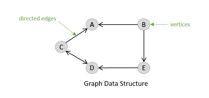
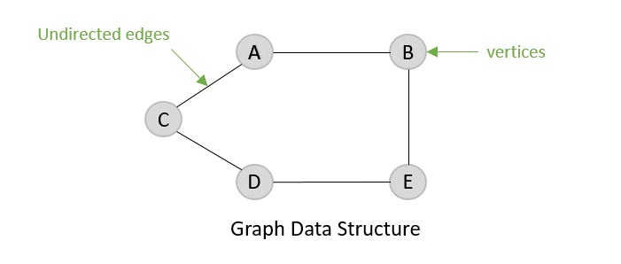
Strongly Connected Components (SCCs) are specific sub-graphs in a directed graph where every node can reach every other node within that sub-graph. In simple terms, SCCs are clusters of nodes that are tightly connected but are separate from other parts of the graph. Understanding SCCs is important, as they help in detecting cycles and studying network structures.

A directed graph is said to be strongly connected if every node can reach every other node directly or indirectly. However, in larger graphs, we may have multiple strongly connected parts that are not connected to each other. These independent sections are called strongly connected components.

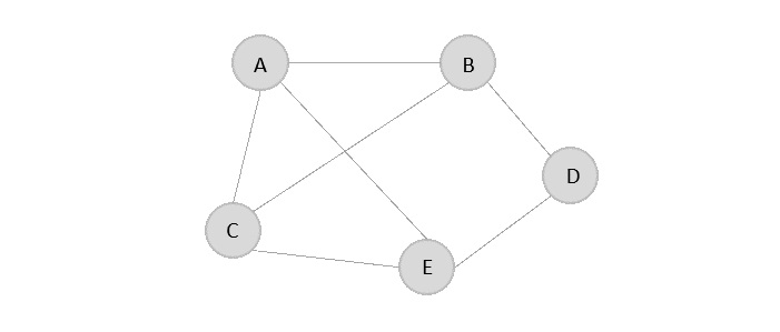
For example, consider a directed graph with nodes A, B, C, D, and E. If A can reach B and B can reach A, but C, D, and E form a separate cluster where they can all reach each other but not A or B, then there are two SCCs in the graph: {A, B} and {C, D, E}.

Strongly Connected Components Algorithm

There are two popular algorithms to find strongly connected components in a graph:

• Kosaraju’s Algorithm
• Tarjan’s Algorithm

Kosaraju’s Algorithm

Kosaraju’s Algorithm is a two-pass algorithm that finds strongly connected components in a directed graph. Here’s how it works:

• First Pass: Perform a Depth First Search (DFS) on the graph and store the order of nodes based on their finishing times.
• Second Pass: Reverse the graph and perform another DFS on the nodes in the order of their finishing times from the first pass. This will give us the strongly connected components.

Kosaraju’s Algorithm Example

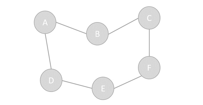
Let’s consider a directed graph with nodes A, B, C, D, and E, and the following edges:

   A -> B
   B -> C
   C -> A
   C -> D
   D -> E
   E -> D

Using Kosaraju’s Algorithm, we can find the strongly connected components in the graph:

• First Pass: The finishing times of the nodes are E, D, C, B, A.
• Second Pass: The strongly connected components are {A, B, C} and {D, E}.

Code for Kosaraju’s Algorithm

Here’s an example code snippet for Kosaraju’s Algorithm in C, C++, Java, and Python:

CC++JavaPython

#include <stdio.h>#include <stdlib.h>#include <string.h>#define MAX_VERTICES 5// Graph adjacency matrixint adj[MAX_VERTICES][MAX_VERTICES]={{0,1,0,0,0},{0,0,1,0,0},{1,0,0,1,0},{0,0,0,0,1},{0,0,0,1,0}};int visited[MAX_VERTICES]={0};int finishing_time[MAX_VERTICES];int finish_index =0;// Mapping index to letters (A-E)char map[MAX_VERTICES]={'A','B','C','D','E'};voidDFS(int vertex,int print){
   visited[vertex]=1;if(print)printf("%c ", map[vertex]);// Print vertex if it's in SCC traversalfor(int v =0; v < MAX_VERTICES; v++){if(adj[vertex][v]&&!visited[v]){DFS(v, print);}}if(!print) finishing_time[finish_index++]= vertex;// Store finishing time if not printing SCC}voidreverse_graph(){int temp[MAX_VERTICES][MAX_VERTICES];for(int i =0; i < MAX_VERTICES; i++){for(int j =0; j < MAX_VERTICES; j++){
         temp[i][j]= adj[i][j];}}// Transpose the graphfor(int i =0; i < MAX_VERTICES; i++){for(int j =0; j < MAX_VERTICES; j++){
         adj[i][j]= temp[j][i];}}}voidfind_scc(){// Step 1: Compute finishing times in the original graphfor(int v =0; v < MAX_VERTICES; v++){if(!visited[v]){DFS(v,0);// First pass DFS (store finish times)}}// Step 2: Reverse the graphreverse_graph();// Step 3: Second DFS based on decreasing finishing timesmemset(visited,0,sizeof(visited));// Reset visited arrayprintf("Strongly Connected Components:\n");for(int i = MAX_VERTICES -1; i >=0; i--){int vertex = finishing_time[i];if(!visited[vertex]){printf("SCC: ");DFS(vertex,1);// Second pass DFS (print SCC)printf("\n");}}}intmain(){find_scc();return0;}

Output

Following is the output of the above code:

Strongly Connected Components:
SCC: A C B
SCC: D E

Tarjan’s Algorithm

Tarjan’s Algorithm is another popular algorithm to find strongly connected components in a directed graph. It uses Depth First Search (DFS) to traverse the graph and identify SCCs. Here’s how it works:

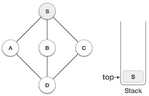
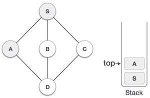
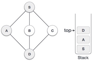
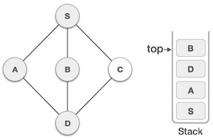
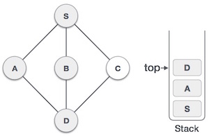
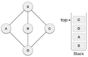
• Initialize a stack to keep track of visited nodes and their order of traversal.
• Perform a DFS traversal of the graph, assigning a unique ID to each node and keeping track of the lowest ID reachable from that node.
• Nodes with the same ID and low-link value form a strongly connected component.

Tarjan’s Algorithm Example

Consider the same directed graph with nodes A, B, C, D, and E, and the following edges:

   A -> B
   B -> C
   C -> A
   C -> D
   D -> E
   E -> D

Using Tarjan’s Algorithm, we can find the strongly connected components in the graph:

• The strongly connected components are {A, B, C} and {D, E}.

Code for Tarjan’s Algorithm

Here’s an example code snippet for Tarjan’s Algorithm in C, C++, Java, and Python:

CC++JavaPython

#include <stdio.h>#include <stdlib.h>#include <string.h>#define MAX_VERTICES 5// Graph adjacency matrixint adj[MAX_VERTICES][MAX_VERTICES]={{0,1,0,0,0},{0,0,1,0,0},{1,0,0,1,0},{0,0,0,0,1},{0,0,0,1,0}};int visited[MAX_VERTICES]={0};int stack[MAX_VERTICES];int stack_index =0;int ids[MAX_VERTICES];int low[MAX_VERTICES];int id =0;// Mapping index to letters (A-E)char map[MAX_VERTICES]={'A','B','C','D','E'};int map_index =0;voidDFS(int vertex){
   stack[stack_index++]= vertex;
   visited[vertex]=1;
   ids[vertex]= low[vertex]= id++;for(int v =0; v < MAX_VERTICES; v++){if(adj[vertex][v]){if(!visited[v]){DFS(v);}if(ids[v]!=-1){
            low[vertex]= low[vertex]0){int node = stack[--stack_index];
         low[node]= ids[vertex];printf("%c ", map[node]);if(node == vertex)break;}printf("\n");}}voidfind_scc(){memset(ids,-1,sizeof(ids));memset(low,-1,sizeof(low));for(int v =0; v < MAX_VERTICES; v++){if(!visited[v]){DFS(v);}}}intmain(){find_scc();return0;}

Output

Following is the output of the above code:

SCC: E D
SCC: C B A

Applications of Strongly Connected Components

Following are some common applications of Strongly Connected Components:

• Network Analysis: SCCs help in understanding the structure and connectivity of networks, such as social networks, transportation networks, and communication networks.
• Graph Algorithms: SCCs are used in various graph algorithms, such as cycle detection, pathfinding, and network flow optimization.
• Software Engineering: SCCs are useful in software engineering for dependency analysis, module identification, and code refactoring.

Conclusion

Understanding Strongly Connected Components is essential for analyzing the connectivity and structure of directed graphs. Algorithms like Kosaraju’s Algorithm and Tarjan’s Algorithm provide efficient ways to identify SCCs in graphs, enabling various applications in network analysis, graph algorithms, and software engineering.

Topological sorting is a way of arranging the nodes of a Directed Acyclic Graph (DAG) in a line, making sure that for every directed edge from u to v, node u comes before v. If the graph has cycles, topological sorting isn’t possible.

In topological sorting, if theres an edge from u to v, u should come before v in the order. Its different from DFS, where we visit a node and then explore its neighbors. In topological sorting, a node should be printed before any of its connected nodes.

Now, lets understand Directed Acyclic Graphs (DAGs). A directed graph has edges that go from one node to another in a specific direction. It is called acyclic if there are no cyclesmeaning theres no way to start from a node and return to it by following edges.

Topological sorting only works for DAGs. If theres a cycle in the graph, we cant arrange the nodes in a proper order because some nodes will keep pointing back, making a valid linear order impossible.

Topological Sort Algorithm

Topological sorting can be done using Depth First Search (DFS) algorithm. The algorithm follows the following steps:

Algorithm

Following are the steps to perform topological sorting using DFS:

• Call the DFS function for a vertex u.
• In the DFS function, mark the vertex u as visited.
• For every adjacent vertex v of u, if v is not visited, then call the DFS function for vertex v.
• After visiting all the adjacent vertices of vertex u, add the vertex u to the topological order list.

After performing the above steps for all the vertices, the topological order list will have the vertices in topological order.

Code for Topological Sort

Let’s see the code for topological sorting using Depth First Search (DFS) algorithm:

CC++JavaPython

#include <stdio.h>#define MAX_VERTICES 6int adj[MAX_VERTICES][MAX_VERTICES]={{0,1,1,0,0,0},{0,0,0,1,1,0},{0,0,0,0,1,0},{0,0,0,0,0,1},{0,0,0,0,0,1},{0,0,0,0,0,0}};int visited[MAX_VERTICES]={0};int topological_order[MAX_VERTICES];int order_index = MAX_VERTICES -1;voidDFS(int vertex){
   visited[vertex]=1;for(int v =0; v < MAX_VERTICES; v++){if(adj[vertex][v]&&!visited[v]){DFS(v);}}
   topological_order[order_index--]= vertex;}voidtopological_sort(){for(int v =0; v < MAX_VERTICES; v++){if(!visited[v]){DFS(v);}}}voidprint_topological_order(){printf("Topological Order: ");for(int i =0; i < MAX_VERTICES; i++){printf("%d ", topological_order[i]);}printf("\n");}intmain(){topological_sort();print_topological_order();return0;}

Output

Following is the output of the above code:

Topological Order: 0 2 1 3 4 5

Time Complexity of Topological Sort

When using Depth First Search (DFS) for topological sorting, the time complexity is O(V + E), where V is the number of vertices and E is the number of edges in the graph. This is because we visit each node once and explore all its edges.

Applications of Topological Sort

Topological sorting has many applications in various fields. Some of the applications of topological sort are:

• Task Scheduling: Used to schedule tasks based on dependencies. Each task is a node, and dependencies are edges. This ensures tasks are executed in the correct order.
• Course Prerequisites: Helps in deciding the order of taking courses. Courses are nodes, and prerequisites are edges, ensuring prerequisites are completed first.
• Build Systems: Used in software build processes to determine the correct sequence for compiling files based on dependencies.
• Network Routing: Helps in routing packets through a network by determining the correct order of processing based on connections between routers.

What is Spanning Tree?

A spanning tree is a subset of Graph G, which has all the vertices covered with minimum possible number of edges. Hence, a spanning tree does not have cycles and it cannot be disconnected..

By this definition, we can draw a conclusion that every connected and undirected Graph G has at least one spanning tree. A disconnected graph does not have any spanning tree, as it cannot be spanned to all its vertices.

We found three spanning trees off one complete graph. A complete undirected graph can have maximum n^n-2 number of spanning trees, where n is the number of nodes. In the above addressed example, n is 3, hence 3³⁻² = 3 spanning trees are possible.

General Properties of Spanning Tree

We now understand that one graph can have more than one spanning tree. Following are a few properties of the spanning tree connected to graph G −

• A connected graph G can have more than one spanning tree.
• All possible spanning trees of graph G, have the same number of edges and vertices.
• The spanning tree does not have any cycle (loops).
• Removing one edge from the spanning tree will make the graph disconnected, i.e. the spanning tree is minimally connected.
• Adding one edge to the spanning tree will create a circuit or loop, i.e. the spanning tree is maximally acyclic.

Mathematical Properties of Spanning Tree

• Spanning tree has n-1 edges, where n is the number of nodes (vertices).
• From a complete graph, by removing maximum e – n + 1 edges, we can construct a spanning tree.
• A complete graph can have maximum n^n-2 number of spanning trees.

Thus, we can conclude that spanning trees are a subset of connected Graph G and disconnected graphs do not have spanning tree.

Application of Spanning Tree

Spanning tree is basically used to find a minimum path to connect all nodes in a graph. Common application of spanning trees are −

• Civil Network Planning
• Computer Network Routing Protocol
• Cluster Analysis

Let us understand this through a small example. Consider, city network as a huge graph and now plans to deploy telephone lines in such a way that in minimum lines we can connect to all city nodes. This is where the spanning tree comes into picture.

Minimum Spanning Tree (MST)

In a weighted graph, a minimum spanning tree is a spanning tree that has minimum weight than all other spanning trees of the same graph. In real-world situations, this weight can be measured as distance, congestion, traffic load or any arbitrary value denoted to the edges.

Minimum Spanning-Tree Algorithm

We shall learn about two most important spanning tree algorithms here −

• Kruskal’s Algorithm
• Prim’s Algorithm

These two algorithms are Greedy algorithms.

Breadth First Search (BFS) Algorithm

Breadth First Search (BFS) algorithm traverses a graph in a breadthward motion to search a graph data structure for a node that meets a set of criteria. It uses a queue to remember the next vertex to start a search, when a dead end occurs in any iteration.

Breadth First Search (BFS) algorithm starts at the tree root and explores all nodes at the present depth prior to moving on to the nodes at the next depth level.

As in the example given above, BFS algorithm traverses from A to B to E to F first then to C and G lastly to D. It employs the following rules.

• Rule 1 − Visit the adjacent unvisited vertex. Mark it as visited. Display it. Insert it in a queue.
• Rule 2 − If no adjacent vertex is found, remove the first vertex from the queue.
• Rule 3 − Repeat Rule 1 and Rule 2 until the queue is empty.

Step	Traversal	Description
1		Initialize the queue.
2		We start from visiting S (starting node), and mark it as visited.
3		We then see an unvisited adjacent node from S. In this example, we have three nodes but alphabetically we choose A, mark it as visited and enqueue it.
4		Next, the unvisited adjacent node from S is B. We mark it as visited and enqueue it.
5		Next, the unvisited adjacent node from S is C. We mark it as visited and enqueue it.
6		Now, S is left with no unvisited adjacent nodes. So, we dequeue and find A.
7		From A we have D as unvisited adjacent node. We mark it as visited and enqueue it.

At this stage, we are left with no unmarked (unvisited) nodes. But as per the algorithm we keep on dequeuing in order to get all unvisited nodes. When the queue gets emptied, the program is over.

Example

Following are the implementations of Breadth First Search (BFS) Algorithm in various programming languages −

CC++JavaPython

#include <stdio.h>#include <stdlib.h>#include <stdbool.h>#define MAX 5structVertex{char label;
   bool visited;};//queue variablesint queue[MAX];int rear =-1;int front =0;int queueItemCount =0;//graph variables//array of verticesstructVertex* lstVertices[MAX];//adjacency matrixint adjMatrix[MAX][MAX];//vertex countint vertexCount =0;//queue functionsvoidinsert(int data){
   queue[++rear]= data;
   queueItemCount++;}intremoveData(){
   queueItemCount--;return queue[front++];}
bool isQueueEmpty(){return queueItemCount ==0;}//graph functions//add vertex to the vertex listvoidaddVertex(char label){structVertex* vertex =(structVertex*)malloc(sizeof(structVertex));
   vertex->label = label;  
   vertex->visited = false;     
   lstVertices[vertexCount++]= vertex;}//add edge to edge arrayvoidaddEdge(int start,int end){
   adjMatrix[start][end]=1;
   adjMatrix[end][start]=1;}//display the vertexvoiddisplayVertex(int vertexIndex){printf("%c ",lstVertices[vertexIndex]->label);}//get the adjacent unvisited vertexintgetAdjUnvisitedVertex(int vertexIndex){int i;for(i =0; i<vertexCount; i++){if(adjMatrix[vertexIndex][i]==1&& lstVertices[i]->visited == false)return i;}return-1;}voidbreadthFirstSearch(){int i;//mark first node as visited
   lstVertices[0]->visited = true;//display the vertexdisplayVertex(0);//insert vertex index in queueinsert(0);int unvisitedVertex;while(!isQueueEmpty()){//get the unvisited vertex of vertex which is at front of the queueint tempVertex =removeData();//no adjacent vertex foundwhile((unvisitedVertex =getAdjUnvisitedVertex(tempVertex))!=-1){    
         lstVertices[unvisitedVertex]->visited = true;displayVertex(unvisitedVertex);insert(unvisitedVertex);}}//queue is empty, search is complete, reset the visited flag        for(i =0;i<vertexCount;i++){
      lstVertices[i]->visited = false;}}intmain(){int i, j;for(i =0; i<MAX; i++){// set adjacency for(j =0; j<MAX; j++)// matrix to 0
         adjMatrix[i][j]=0;}addVertex('S');// 0addVertex('A');// 1addVertex('B');// 2addVertex('C');// 3addVertex('D');// 4addEdge(0,1);// S - AaddEdge(0,2);// S - BaddEdge(0,3);// S - CaddEdge(1,4);// A - DaddEdge(2,4);// B - DaddEdge(3,4);// C - Dprintf("\nBreadth First Search: ");breadthFirstSearch();return0;}

Output

Breadth First Search: S A B C D

Click to check C implementation of Breadth First Search (BFS) Algorithm

Complexity of BFS Algorithm

Time Complexity

The time complexity of the BFS algorithm is represented in the form of O(V + E), where V is the number of nodes and E is the number of edges.

Space Complexity

The space complexity of the BFS algorithm is O(V).

Depth First Search (DFS) Algorithm

Depth First Search (DFS) algorithm is a recursive algorithm for searching all the vertices of a graph or tree data structure. This algorithm traverses a graph in a depthward motion and uses a stack to remember to get the next vertex to start a search, when a dead end occurs in any iteration.

As in the example given above, DFS algorithm traverses from S to A to D to G to E to B first, then to F and lastly to C. It employs the following rules.

• Rule 1 − Visit the adjacent unvisited vertex. Mark it as visited. Display it. Push it in a stack.
• Rule 2 − If no adjacent vertex is found, pop up a vertex from the stack. (It will pop up all the vertices from the stack, which do not have adjacent vertices.)
• Rule 3 − Repeat Rule 1 and Rule 2 until the stack is empty.

Step	Traversal	Description
1		Initialize the stack.
2		Mark S as visited and put it onto the stack. Explore any unvisited adjacent node from S. We have three nodes and we can pick any of them. For this example, we shall take the node in an alphabetical order.
3		Mark A as visited and put it onto the stack. Explore any unvisited adjacent node from A. Both S and D are adjacent to A but we are concerned for unvisited nodes only.
4		Visit D and mark it as visited and put onto the stack. Here, we have B and C nodes, which are adjacent to D and both are unvisited. However, we shall again choose in an alphabetical order.
5		We choose B, mark it as visited and put onto the stack. Here B does not have any unvisited adjacent node. So, we pop B from the stack.
6		We check the stack top for return to the previous node and check if it has any unvisited nodes. Here, we find D to be on the top of the stack.
7		Only unvisited adjacent node is from D is C now. So we visit C, mark it as visited and put it onto the stack.

As C does not have any unvisited adjacent node so we keep popping the stack until we find a node that has an unvisited adjacent node. In this case, there’s none and we keep popping until the stack is empty.

Example

Following are the implementations of Depth First Search (DFS) Algorithm in various programming languages −

CC++JavaPython

#include <stdio.h>#include <stdlib.h>#include <stdbool.h>#define MAX 5structVertex{char label;
   bool visited;};//stack variablesint stack[MAX];int top =-1;//graph variables//array of verticesstructVertex* lstVertices[MAX];//adjacency matrixint adjMatrix[MAX][MAX];//vertex countint vertexCount =0;//stack functionsvoidpush(int item){ 
   stack[++top]= item;}intpop(){return stack[top--];}intpeek(){return stack[top];}
bool isStackEmpty(){return top ==-1;}//graph functions//add vertex to the vertex listvoidaddVertex(char label){structVertex* vertex =(structVertex*)malloc(sizeof(structVertex));
   vertex->label = label;  
   vertex->visited = false;     
   lstVertices[vertexCount++]= vertex;}//add edge to edge arrayvoidaddEdge(int start,int end){
   adjMatrix[start][end]=1;
   adjMatrix[end][start]=1;}//display the vertexvoiddisplayVertex(int vertexIndex){printf("%c ",lstVertices[vertexIndex]->label);}//get the adjacent unvisited vertexintgetAdjUnvisitedVertex(int vertexIndex){int i;for(i =0; i < vertexCount; i++){if(adjMatrix[vertexIndex][i]==1&& lstVertices[i]->visited == false){return i;}}return-1;}voiddepthFirstSearch(){int i;//mark first node as visited
   lstVertices[0]->visited = true;//display the vertexdisplayVertex(0);//push vertex index in stackpush(0);while(!isStackEmpty()){//get the unvisited vertex of vertex which is at top of the stackint unvisitedVertex =getAdjUnvisitedVertex(peek());//no adjacent vertex foundif(unvisitedVertex ==-1){pop();}else{
         lstVertices[unvisitedVertex]->visited = true;displayVertex(unvisitedVertex);push(unvisitedVertex);}}//stack is empty, search is complete, reset the visited flag        for(i =0;i < vertexCount;i++){
      lstVertices[i]->visited = false;}}intmain(){int i, j;for(i =0; i < MAX; i++){// set adjacencyfor(j =0; j < MAX; j++)// matrix to 0
         adjMatrix[i][j]=0;}addVertex('S');// 0addVertex('A');// 1addVertex('B');// 2addVertex('C');// 3addVertex('D');// 4addEdge(0,1);// S - AaddEdge(0,2);// S - BaddEdge(0,3);// S - CaddEdge(1,4);// A - DaddEdge(2,4);// B - DaddEdge(3,4);// C - Dprintf("Depth First Search: ");depthFirstSearch();return0;}

Output

Depth First Search: S A D B C

Click to check C implementation of Depth First Search (BFS) Algorithm

Complexity of DFS Algorithm

Time Complexity

The time complexity of the DFS algorithm is represented in the form of O(V + E), where V is the number of nodes and E is the number of edges.

Space Complexity

The space complexity of the DFS algorithm is O(V).

What is a Graph?

A graph is an abstract data type (ADT) which consists of a set of objects that are connected to each other via links. The interconnected objects are represented by points termed as vertices, and the links that connect the vertices are called edges.

Formally, a graph is a pair of sets (V, E), where V is the set of vertices and E is the set of edges, connecting the pairs of vertices. Take a look at the following graph −

In the above graph,

V = {a, b, c, d, e}

E = {ab, ac, bd, cd, de}

Graph Data Structure

Mathematical graphs can be represented in data structure. We can represent a graph using an array of vertices and a two-dimensional array of edges. Before we proceed further, let’s familiarize ourselves with some important terms −

• Vertex − Each node of the graph is represented as a vertex. In the following example, the labeled circle represents vertices. Thus, A to G are vertices. We can represent them using an array as shown in the following image. Here A can be identified by index 0. B can be identified using index 1 and so on.
• Edge − Edge represents a path between two vertices or a line between two vertices. In the following example, the lines from A to B, B to C, and so on represents edges. We can use a two-dimensional array to represent an array as shown in the following image. Here AB can be represented as 1 at row 0, column 1, BC as 1 at row 1, column 2 and so on, keeping other combinations as 0.
• Adjacency − Two node or vertices are adjacent if they are connected to each other through an edge. In the following example, B is adjacent to A, C is adjacent to B, and so on.
• Path − Path represents a sequence of edges between the two vertices. In the following example, ABCD represents a path from A to D.

Operations of Graphs

The primary operations of a graph include creating a graph with vertices and edges, and displaying the said graph. However, one of the most common and popular operation performed using graphs are Traversal, i.e. visiting every vertex of the graph in a specific order.

There are two types of traversals in Graphs −

• Depth First Search Traversal
• Breadth First Search Traversal

Depth First Search Traversal

Depth First Search is a traversal algorithm that visits all the vertices of a graph in the decreasing order of its depth. In this algorithm, an arbitrary node is chosen as the starting point and the graph is traversed back and forth by marking unvisited adjacent nodes until all the vertices are marked.

The DFS traversal uses the stack data structure to keep track of the unvisited nodes.

Click and check Depth First Search Traversal

Breadth First Search Traversal

Breadth First Search is a traversal algorithm that visits all the vertices of a graph present at one level of the depth before moving to the next level of depth. In this algorithm, an arbitrary node is chosen as the starting point and the graph is traversed by visiting the adjacent vertices on the same depth level and marking them until there is no vertex left.

The DFS traversal uses the queue data structure to keep track of the unvisited nodes.

Click and check Breadth First Search Traversal

Representation of Graphs

While representing graphs, we must carefully depict the elements (vertices and edges) present in the graph and the relationship between them. Pictorially, a graph is represented with a finite set of nodes and connecting links between them. However, we can also represent the graph in other most commonly used ways, like −

• Adjacency Matrix
• Adjacency List

Adjacency Matrix

The Adjacency Matrix is a V x V matrix where the values are filled with either 0 or 1. If the link exists between Vi and Vj, it is recorded 1; otherwise, 0.

For the given graph below, let us construct an adjacency matrix −

The adjacency matrix is −

Adjacency List

The adjacency list is a list of the vertices directly connected to the other vertices in the graph.

The adjacency list is −

Types of graph

There are two basic types of graph −

• Directed Graph
• Undirected Graph

Directed graph, as the name suggests, consists of edges that possess a direction that goes either away from a vertex or towards the vertex. Undirected graphs have edges that are not directed at all.

Directed Graph

Undirected Graph

Spanning Tree

A spanning tree is a subset of an undirected graph that contains all the vertices of the graph connected with the minimum number of edges in the graph. Precisely, the edges of the spanning tree is a subset of the edges in the original graph.

If all the vertices are connected in a graph, then there exists at least one spanning tree. In a graph, there may exist more than one spanning tree.

Properties

• A spanning tree does not have any cycle.
• Any vertex can be reached from any other vertex.

Example

In the following graph, the highlighted edges form a spanning tree.

Minimum Spanning Tree

A Minimum Spanning Tree (MST) is a subset of edges of a connected weighted undirected graph that connects all the vertices together with the minimum possible total edge weight. To derive an MST, Prim’s algorithm or Kruskal’s algorithm can be used. Hence, we will discuss Prim’s algorithm in this chapter.

As we have discussed, one graph may have more than one spanning tree. If there are n number of vertices, the spanning tree should have n − l1 number of edges. In this context, if each edge of the graph is associated with a weight and there exists more than one spanning tree, we need to find the minimum spanning tree of the graph.

Moreover, if there exist any duplicate weighted edges, the graph may have multiple minimum spanning tree.

In the above graph, we have shown a spanning tree though it’s not the minimum spanning tree. The cost of this spanning tree is (5+7+3+3+5+8+3+4)=38.

Shortest Path

The shortest path in a graph is defined as the minimum cost route from one vertex to another. This is most commonly seen in weighted directed graphs but are also applicable to undirected graphs.

A popular real−world application of finding the shortest path in a graph is a map. Navigation is made easier and simpler with the various shortest path algorithms where destinations are considered vertices of the graph and routes are the edges. The two common shortest path algorithms are −

• Dijkstra’s Shortest Path Algorithm
• Bellman Ford’s Shortest Path Algorithm

Example

Following are the implementations of this operation in various programming languages −

CC++JavaPython

#include <stdio.h>#include <stdlib.h>#include <stdlib.h>#define V 5 // Maximum number of vertices in the graphstructgraph{// declaring graph data structurestructvertex*point[V];};structvertex{// declaring verticesint end;structvertex*next;};structEdge{// declaring edgesint end, start;};structgraph*create_graph(structEdge edges[],int x){int i;structgraph*graph =(structgraph*)malloc(sizeof(structgraph));for(i =0; i < V; i++){
      graph->point[i]=NULL;}for(i =0; i < x; i++){int start = edges[i].start;int end = edges[i].end;structvertex*v =(structvertex*)malloc(sizeof(structvertex));
      v->end = end;
      v->next = graph->point[start];
      graph->point[start]= v;}return graph;}intmain(){structEdge edges[]={{0,1},{0,2},{0,3},{1,2},{1,4},{2,4},{2,3},{3,1}};int n =sizeof(edges)/sizeof(edges[0]);structgraph*graph =create_graph(edges, n);printf("The graph created is: ");for(int i =0; i < V; i++){structvertex*ptr = graph->point[i];while(ptr !=NULL){printf("(%d -> %d)\t", i, ptr->end);
         ptr = ptr->next;}printf("\n");}return0;}

Output

The graph created is:
(1 -> 3)	(1 -> 0)	
(2 -> 1)	(2 -> 0)	
(3 -> 2)	(3 -> 0)	
(4 -> 2)	(4 -> 1)