The Naive Bayes algorithm is a classification algorithm based on Bayes’ theorem. The algorithm assumes that the features are independent of each other, which is why it is called “naive.” It calculates the probability of a sample belonging to a particular class based on the probabilities of its features. For example, a phone may be considered as smart if it has touch-screen, internet facility, good camera, etc. Even if all these features are dependent on each other, but all these features independently contribute to the probability of that the phone is a smart phone.
In Bayesian classification, the main interest is to find the posterior probabilities i.e. the probability of a label given some observed features, P(L | features). With the help of Bayes theorem, we can express this in quantitative form as follows −
P(L|features)=P(L)P(features|L)P(features)
Here,
P(L|features) is the posterior probability of class.
P(L) is the prior probability of class.
P(features|L) is the likelihood which is the probability of predictor given class.
P(features) is the prior probability of predictor.
In the Naive Bayes algorithm, we use Bayes’ theorem to calculate the probability of a sample belonging to a particular class. We calculate the probability of each feature of the sample given the class and multiply them to get the likelihood of the sample belonging to the class. We then multiply the likelihood with the prior probability of the class to get the posterior probability of the sample belonging to the class. We repeat this process for each class and choose the class with the highest probability as the class of the sample.
Types of Naive Bayes Algorithm
There are many types of Naive Bayes Algorithm. Here we discuss the following three types −
Gaussian Nave Bayes
Gaussian Nave Bayes is the simplest Nave Bayes classifier having the assumption that the data from each label is drawn from a simple Gaussian distribution. It is used when the features are continuous variables that follow a normal distribution.
Multinomial Nave Bayes
Another useful Nave Bayes classifier is Multinomial Nave Bayes in which the features are assumed to be drawn from a simple Multinomial distribution. Such kind of Nave Bayes are most appropriate for the features that represents discrete counts. It is commonly used in text classification tasks where the features are the frequency of words in a document.
Bernoulli Nave Bayes
Another important model is Bernoulli Nave Bayes in which features are assumed to be binary (0s and 1s). Text classification with ‘bag of words’ model can be an application of Bernoulli Nave Bayes.
Implementation of Nave Bayes Algorithm in Python
Depending on our data set, we can choose any of the Nave Bayes model explained above. Here, we are implementing Gaussian Nave Bayes model in Python −
We will start with required imports as follows −
import numpy as np
import matplotlib.pyplot as plt
import seaborn as sns; sns.set()
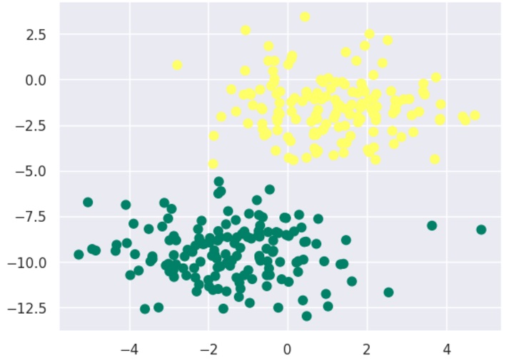
Now, by using make_blobs() function of Scikit learn, we can generate blobs of points with Gaussian distribution as follows −
from sklearn.datasets import make_blobs
X, y = make_blobs(300,2, centers=2, random_state=2, cluster_std=1.5)
plt.scatter(X[:,0], X[:,1], c=y, s=50, cmap='summer');
Next, for using GaussianNB model, we need to import and make its object as follows −
from sklearn.naive_bayes import GaussianNB
model_GNB = GaussianNB()
model_GNB.fit(X, y);
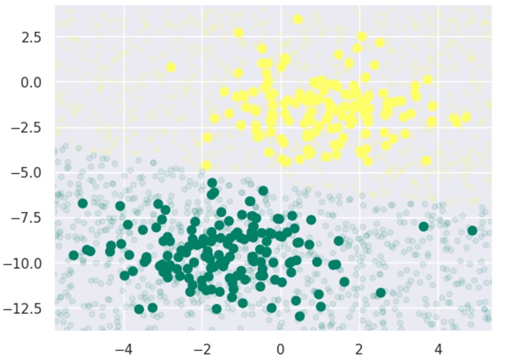
Now, we have to do prediction. It can be done after generating some new data as follows −
Let’s discuss some of the advantages and limitations of Naive Bayes classification algorithm.
Pros
The followings are some pros of using Nave Bayes classifiers −
Nave Bayes classification is easy to implement and fast.
It will converge faster than discriminative models like logistic regression.
It requires less training data.
It is highly scalable in nature, or they scale linearly with the number of predictors and data points.
It can make probabilistic predictions and can handle continuous as well as discrete data.
Nave Bayes classification algorithm can be used for binary as well as multi-class classification problems both.
Cons
The followings are some cons of using Nave Bayes classifiers −
One of the most important cons of Nave Bayes classification is its strong feature independence because in real life it is almost impossible to have a set of features which are completely independent of each other.
Another issue with Nave Bayes classification is its ‘zero frequency’ which means that if a categorial variable has a category but not being observed in training data set, then Nave Bayes model will assign a zero probability to it and it will be unable to make a prediction.
Applications of Nave Bayes classification
The following are some common applications of Nave Bayes classification −
Real-time prediction − Due to its ease of implementation and fast computation, it can be used to do prediction in real-time.
Multi-class prediction − Nave Bayes classification algorithm can be used to predict posterior probability of multiple classes of target variable.
Text classification − Due to the feature of multi-class prediction, Nave Bayes classification algorithms are well suited for text classification. That is why it is also used to solve problems like spam-filtering and sentiment analysis.
Recommendation system − Along with the algorithms like collaborative filtering, Nave Bayes makes a Recommendation system which can be used to filter unseen information and to predict weather a user would like the given resource or not.
K-nearest neighbors (KNN) algorithm is a type of supervised ML algorithm which can be used for both classification as well as regression predictive problems. However, it is mainly used for classification predictive problems in industry. The main idea behind KNN is to find the k-nearest data points to a given test data point and use these nearest neighbors to make a prediction. The value of k is a hyperparameter that needs to be tuned, and it represents the number of neighbors to consider.
For classification problems, the KNN algorithm assigns the test data point to the class that appears most frequently among the k-nearest neighbors. In other words, the class with the highest number of neighbors is the predicted class.
For regression problems, the KNN algorithm assigns the test data point the average of the k-nearest neighbors’ values.
The distance metric used to measure the similarity between two data points is an essential factor that affects the KNN algorithm’s performance. The most commonly used distance metrics are Euclidean distance, Manhattan distance, and Minkowski distance.
The following two properties would define KNN well −
Lazy learning algorithm − KNN is a lazy learning algorithm because it does not have a specialized training phase and uses all the data for training while classification.
Non-parametric learning algorithm − KNN is also a non-parametric learning algorithm because it doesn’t assume anything about the underlying data.
How Does K-Nearest Neighbors Algorithm Work?
K-nearest neighbors (KNN) algorithm uses ‘feature similarity’ to predict the values of new datapoints which further means that the new data point will be assigned a value based on how closely it matches the points in the training set. We can understand its working with the help of following steps −
Step 1 − For implementing any algorithm, we need dataset. So during the first step of KNN, we must load the training as well as test data.
Step 2 − Next, we need to choose the value of K i.e. the nearest data points. K can be any integer.
Step 3 − For each point in the test data do the following −3.1 − Calculate the distance between test data and each row of training data with the help of any of the method namely: Euclidean, Manhattan or Hamming distance. The most commonly used method to calculate distance is Euclidean.3.2 − Now, based on the distance value, sort them in ascending order.3.3 − Next, it will choose the top K rows from the sorted array.3.4 − Now, it will assign a class to the test point based on most frequent class of these rows.
Step 4 − End
Example
The following is an example to understand the concept of K and working of KNN algorithm −
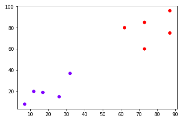
Suppose we have a dataset which can be plotted as follows −
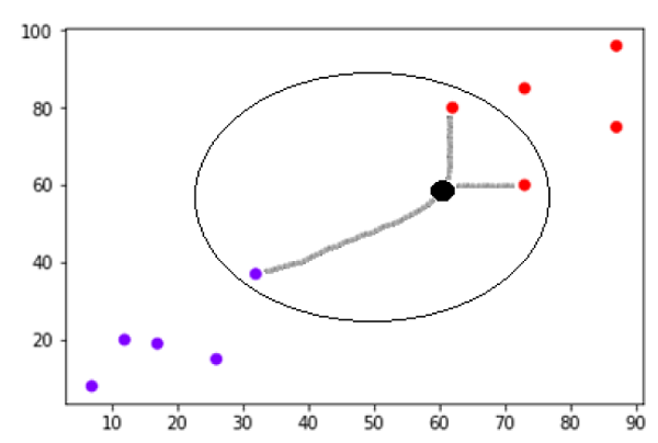
Now, we need to classify new data point with black dot (at point 60,60) into blue or red class. We are assuming K = 3 i.e. it would find three nearest data points. It is shown in the next diagram −
We can see in the above diagram the three nearest neighbors of the data point with black dot. Among those three, two of them lies in Red class hence the black dot will also be assigned in red class.
Building a K Nearest Neighbors Model
We can follow the below steps to build a KNN model −
Load the data − The first step is to load the dataset into memory. This can be done using various libraries such as pandas or numpy.
Split the data − The next step is to split the data into training and test sets. The training set is used to train the KNN algorithm, while the test set is used to evaluate its performance.
Normalize the data − Before training the KNN algorithm, it is essential to normalize the data to ensure that each feature contributes equally to the distance metric calculation.
Calculate distances − Once the data is normalized, the KNN algorithm calculates the distances between the test data point and each data point in the training set.
Select k-nearest neighbors − The KNN algorithm selects the k-nearest neighbors based on the distances calculated in the previous step.
Make a prediction − For classification problems, the KNN algorithm assigns the test data point to the class that appears most frequently among the k-nearest neighbors. For regression problems, the KNN algorithm assigns the test data point the average of the k-nearest neighbors’ values.
Evaluate performance − Finally, the KNN algorithm’s performance is evaluated using various metrics such as accuracy, precision, recall, and F1-score.
Implementation of KNN Algorithm in Python
As we know K-nearest neighbors (KNN) algorithm can be used for both classification as well as regression. The following are the recipes in Python to use KNN as classifier as well as regressor −
KNN as Classifier
First, start with importing necessary python packages −
import numpy as np
import matplotlib.pyplot as plt
import pandas as pd
Next, download the iris dataset from its weblink as follows −
It is very simple algorithm to understand and interpret.
It is very useful for nonlinear data because there is no assumption about data in this algorithm.
It is a versatile algorithm as we can use it for classification as well as regression.
It has relatively high accuracy but there are much better supervised learning models than KNN.
Cons
It is computationally a bit expensive algorithm because it stores all the training data.
High memory storage required as compared to other supervised learning algorithms.
Prediction is slow in case of big N.
It is very sensitive to the scale of data as well as irrelevant features.
Applications of KNN
The following are some of the areas in which KNN can be applied successfully −
Banking System
KNN can be used in banking system to predict weather an individual is fit for loan approval? Does that individual have the characteristics similar to the defaulters one?
Calculating Credit Ratings
KNN algorithms can be used to find an individual’s credit rating by comparing with the persons having similar traits.
Politics
With the help of KNN algorithms, we can classify a potential voter into various classes like “Will Vote”, “Will not Vote”, “Will Vote to Party ‘Congress’, “Will Vote to Party ‘BJP’.
Other areas in which KNN algorithm can be used are Speech Recognition, Handwriting Detection, Image Recognition and Video Recognition.
Logistic regression is a supervised learning classification algorithm used to predict the probability of a target variable. The nature of target or dependent variable is dichotomous, which means there would be only two possible classes.
In simple words, the dependent variable is binary in nature having data coded as either 1 (stands for success/yes) or 0 (stands for failure/no).
Mathematically, a logistic regression model predicts P(Y=1) as a function of X. It is one of the simplest ML algorithms that can be used for various classification problems such as spam detection, Diabetes prediction, cancer detection etc.
Types of Logistic Regression
Generally, logistic regression means binary logistic regression having binary target variables, but there can be two more categories of target variables that can be predicted by it. Based on those number of categories, Logistic regression can be divided into following types −
Binary or Binomial
In such a kind of classification, a dependent variable will have only two possible types either 1 and 0. For example, these variables may represent success or failure, yes or no, win or loss etc.
Multinomial
In such a kind of classification, dependent variable can have 3 or more possible unordered types or the types having no quantitative significance. For example, these variables may represent “Type A” or “Type B” or “Type C”.
Ordinal
In such a kind of classification, dependent variable can have 3 or more possible ordered types or the types having a quantitative significance. For example, these variables may represent “poor” or “good”, “very good”, “Excellent” and each category can have the scores like 0,1,2,3.
Logistic Regression Assumptions
Before diving into the implementation of logistic regression, we must be aware of the following assumptions about the same −
In case of binary logistic regression, the target variables must be binary always and the desired outcome is represented by the factor level 1.
There should not be any multi-collinearity in the model, which means the independent variables must be independent of each other .
We must include meaningful variables in our model.
We should choose a large sample size for logistic regression.
Binary Logistic Regression Model
The simplest form of logistic regression is binary or binomial logistic regression in which the target or dependent variable can have only 2 possible types either 1 or 0. It allows us to model a relationship between multiple predictor variables and a binary/binomial target variable. In case of logistic regression, the linear function is basically used as an input to another function such as in the following relation −
hθ(x)=g(θTx)0hθ1
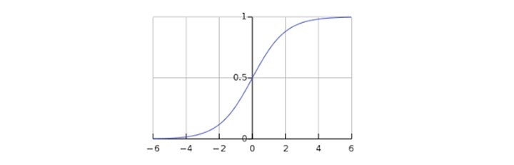
Here, is the logistic or sigmoid function which can be given as follows −
g(z)=11+e−z=θT
To sigmoid curve can be represented with the help of following graph. We can see the values of y-axis lie between 0 and 1 and crosses the axis at 0.5.
The classes can be divided into positive or negative. The output comes under the probability of positive class if it lies between 0 and 1. For our implementation, we are interpreting the output of hypothesis function as positive if it is 0.5, otherwise negative.
We also need to define a loss function to measure how well the algorithm performs using the weights on functions, represented by theta as follows −
=()
J(θ)=1m.(−yTlog(h)−(1−y)Tlog(1−h))
Now, after defining the loss function our prime goal is to minimize the loss function. It can be done with the help of fitting the weights which means by increasing or decreasing the weights. With the help of derivatives of the loss function w.r.t each weight, we would be able to know what parameters should have high weight and what should have smaller weight.
The following gradient descent equation tells us how loss would change if we modified the parameters −
()θj=1mXT(())
Implementation of Binary Logistic Regression Model in Python
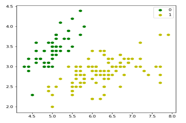
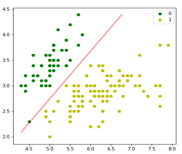
Now we will implement the above concept of binomial logistic regression in Python. For this purpose, we are using a multivariate flower dataset named iris which have 3 classes of 50 instances each, but we will be using the first two feature columns. Every class represents a type of iris flower.
First, we need to import the necessary libraries as follows −
import numpy as np
import matplotlib.pyplot as plt
import seaborn as sns
from sklearn import datasets
Next, load the iris dataset as follows −
iris = datasets.load_iris()
X = iris.data[:,:2]
y =(iris.target !=0)*1
Another useful form of logistic regression is multinomial logistic regression in which the target or dependent variable can have 3 or more possible unordered types i.e. the types having no quantitative significance.
Implementation of Multinomial Logistic Regression Model in Python
Now we will implement the above concept of multinomial logistic regression in Python. For this purpose, we are using a dataset from sklearn named digit.
First, we need to import the necessary libraries as follows −
Import sklearn
from sklearn import datasets
from sklearn import linear_model
from sklearn import metrics
from sklearn.model_selection import train_test_split
Next, we need to load digit dataset −
digits = datasets.load_digits()
Now, define the feature matrix(X) and response vector(y)as follows −
X = digits.data
y = digits.target
With the help of next line of code, we can split X and y into training and testing sets −
X_train, X_test, y_train, y_test = train_test_split(X, y, test_size=0.4, random_state=1)
Now create an object of logistic regression as follows −
digreg = linear_model.LogisticRegression()
Now, we need to train the model by using the training sets as follows −
digreg.fit(X_train, y_train)
Next, make the predictions on testing set as follows −
y_pred = digreg.predict(X_test)
Next print the accuracy of the model as follows −
print("Accuracy of Logistic Regression model is:",
metrics.accuracy_score(y_test, y_pred)*100)
Output
Accuracy of Logistic Regression model is: 95.6884561891516
From the above output we can see the accuracy of our model is around 96 percent.
Classification may be defined as the process of predicting class or category from observed values or given data points. The categorized output can have the form such as “Black” or “White” or “spam” or “no spam”.
Classification in machine learning is a supervised learning technique where an algorithm is trained with labeled data to predict the category of new data.
Mathematically, classification is the task of approximating a mapping function (f) from input variables (X) to output variables (Y). It is basically belongs to the supervised machine learning in which targets are also provided along with the input data set.
An example of classification problem can be the spam detection in emails. There can be only two categories of output, “spam” and “no spam”; hence this is a binary type classification.
To implement this classification, we first need to train the classifier. For this example, “spam” and “no spam” emails would be used as the training data. After successfully train the classifier, it can be used to detect an unknown email.
Types of Learners in Classification
We have two types of learners in respective to classification problems −
Lazy Learners − As the name suggests, such kind of learners waits for the testing data to be appeared after storing the training data. Classification is done only after getting the testing data. They spend less time on training but more time on predicting. Examples of lazy learners are K-nearest neighbor and case-based reasoning.
Eager Learners − As opposite to lazy learners, eager learners construct classification model without waiting for the testing data to be appeared after storing the training data. They spend more time on training but less time on predicting. Examples of eager learners are Decision Trees, Nave Bayes and Artificial Neural Networks (ANN).
Classification Algorithms in Machine Learning
The classification algorithm is a type of supervised learning technique that involves predicting a categorical target variable based on a set of input features. It is commonly used to solve problems such as spam detection, fraud detection, image recognition, sentiment analysis, and many others.
The goal of a classification model is to learn a mapping function (f) between the input features (X) and the target variable (Y). This mapping function is often represented as a decision boundary, which separates different classes in the input feature space. Once the model is trained, it can be used to predict the class of new, unseen examples.
The followings are some important ML classification algorithms −
Logistic Regression
K-Nearest Neighbors (KNN)
Support Vector Machine (SVM)
Decision Tree
Nave Bayes
Random Forest
We will be discussing all these classification algorithms in detail in further chapters. However let’s discuss these algorithms in brief as follows −
Logistic Regression
Logistic Regression is a popular algorithm used for binary classification problems, where the target variable is categorical with two classes. It models the probability of the target variable given the input features and predicts the class with the highest probability.
Logistic regression is a type of generalized linear model, where the target variable follows a Bernoulli distribution. The model consists of a linear function of the input features, which is transformed using the logistic function to produce a probability value between 0 and 1.
K-Nearest Neighbors (KNN)
K-Nearest Neighbors (KNN) is a supervised learning algorithm that can be used for both classification and regression problems. The main idea behind KNN is to find the k-nearest data points to a given test data point and use these nearest neighbors to make a prediction. The value of k is a hyperparameter that needs to be tuned, and it represents the number of neighbors to consider.
For classification problems, the KNN algorithm assigns the test data point to the class that appears most frequently among the k-nearest neighbors. In other words, the class with the highest number of neighbors is the predicted class.
For regression problems, the KNN algorithm assigns the test data point the average of the k-nearest neighbors’ values.
Support Vector Machine (SVM)
Support Vector Machines (SVMs) are powerful yet flexible supervised machine learning algorithm which is used for both classification and regression. But generally, they are used in classification problems. In 1960s, SVMs were first introduced but later they got refined in 1990 also. SVMs have their unique way of implementation as compared to other machine learning algorithms. Now a days, they are extremely popular because of their ability to handle multiple continuous and categorical variables.
Decision Tree
The Decision Tree algorithm is a hierarchical tree-based algorithm that is used to classify or predict outcomes based on a set of rules. It works by splitting the data into subsets based on the values of the input features. The algorithm recursively splits the data until it reaches a point where the data in each subset belongs to the same class or has the same value for the target variable. The resulting tree is a set of decision rules that can be used to make predictions or classify new data.
Nave Bayes
The Nave Bayes algorithm is a classification algorithm based on Bayes’ theorem. The algorithm assumes that the features are independent of each other, which is why it is called “naive.” It calculates the probability of a sample belonging to a particular class based on the probabilities of its features. For example, a phone may be considered as smart if it has touch-screen, internet facility, good camera, etc. Even if all these features are dependent on each other, but all these features independently contribute to the probability of that the phone is a smart phone.
Random Forest
Random Forest is a machine learning algorithm that uses an ensemble of decision trees to make predictions. The algorithm was first introduced by Leo Breiman in 2001. The key idea behind the algorithm is to create a large number of decision trees, each of which is trained on a different subset of the data. The predictions of these individual trees are then combined to produce a final prediction.
Applications of Classification in Machine Learning
Some of the most important applications of classification algorithms are as follows −
Speech Recognition
Handwriting Recognition
Biometric Identification
Document Classification
Image Classification
Spam Filtering
Fraud Detection
Facial Recognition
Building a Classication Model in Machine Learning
Let us now take a look at the steps involved in building a classification model −
1. Data Preparation
The first step is to collect and preprocess the data. This involves cleaning the data, handling missing values, and converting categorical variables to numerical values.
2. Feature Extraction/Selection
The next step is to extract or select relevant features from the data. This is an important step because the quality of the features can greatly impact the performance of the model. Some common feature selection techniques include correlation analysis, feature importance ranking, and principal component analysis.
3. Model Selection
Once the features are selected, the next step is to choose an appropriate classification algorithm. There are many different algorithms to choose from, each with its own strengths and weaknesses. Some popular algorithms include logistic regression, decision trees, random forests, support vector machines, and neural networks
4. Model Training
After selecting a suitable algorithm, the next step is to train the model on the labeled training data. During training, the model learns the mapping function between the input features and the target variable. The model parameters are adjusted iteratively to minimize the difference between the predicted outputs and the actual outputs.
5. Model Evaluation
Once the model is trained, the next step is to evaluate its performance on a separate set of validation data. This is done to estimate the model’s accuracy and generalization performance. Common evaluation metrics include accuracy, precision, recall, F1-score, and area under the receiver operating characteristic (ROC) curve.
5. Hyperparameter Tuning
In many cases, the performance of the model can be further improved by tuning its hyperparameters. Hyperparameters are settings that are chosen before training the model and control aspects such as the learning rate, regularization strength, and the number of hidden layers in a neural network. Grid search, random search, and Bayesian optimization are some common techniques used for hyperparameter tuning.
6. Model Deployment
Once the model has been trained and evaluated, the final step is to deploy it in a production environment. This involves integrating the model into a larger system, testing it on realworld data, and monitoring its performance over time.
Building a Classification Model with Python
Scikit-learn, a Python library for machine learning can be used to build a classifier in Python. The steps for building a classifier in Python are as follows −
Step 1: Importing necessary python package
For building a classifier using scikit-learn, we need to import it. We can import it by using following script −
import sklearn
Step 2: Importing dataset
After importing necessary package, we need a dataset to build classification prediction model. We can import it from sklearn dataset or can use other one as per our requirement. We are going to use sklearns Breast Cancer Wisconsin Diagnostic Database. We can import it with the help of following script −
from sklearn.datasets import load_breast_cancer
The following script will load the dataset;
data = load_breast_cancer()
We also need to organize the data and it can be done with the help of following scripts −
Step 3: Organizing data into training & testing sets
As we need to test our model on unseen data, we will divide our dataset into two parts: a training set and a test set. We can use train_test_split() function of sklearn python package to split the data into sets. The following command will import the function −
from sklearn.model_selection import train_test_split
Now, next command will split the data into training & testing data. In this example, we are using taking 40 percent of the data for testing purpose and 60 percent of the data for training purpose −
After dividing the data into training and testing we need to build the model. We will be using Nave Bayes algorithm for this purpose. The following commands will import the GaussianNB module −
from sklearn.naive_bayes import GaussianNB
Now, initialize the model as follows −
gnb = GaussianNB()
Next, with the help of following command we can train the model −
model = gnb.fit(train, train_labels)
Now, for evaluation purpose we need to make predictions. It can be done by using predict() function as follows −
The above series of 0s and 1s in output are the predicted values for the Malignant and Benign tumor classes.
Step 5: Finding accuracy
We can find the accuracy of the model build in previous step by comparing the two arrays namely test_labels and preds. We will be using the accuracy_score() function to determine the accuracy.
from sklearn.metrics import accuracy_score
print(accuracy_score(test_labels,preds))0.951754385965
The above output shows that NaveBayes classifier is 95.17% accurate.
Evaluation Metrics for Classification Model
The job is not done even if you have finished implementation of your Machine Learning application or model. We must have to find out how effective our model is? There can be different evaluation/ performance metrics, but we must choose it carefully because the choice of metrics influences how the performance of a machine learning algorithm is measured and compared.
The following are some of the important classification evaluation metrics among which you can choose based upon your dataset and kind of problem −
Confusion Matrix
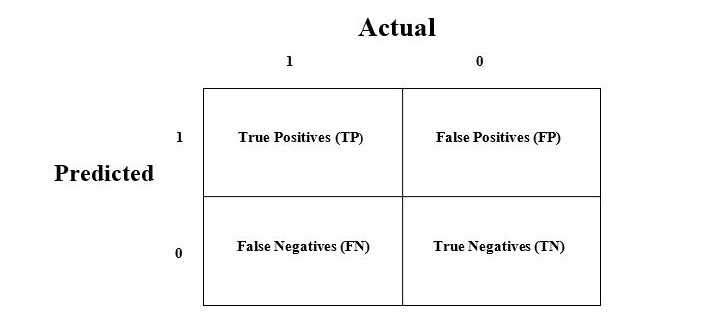
The confusion matrix is the easiest way to measure the performance of a classification problem where the output can be of two or more type of classes. A confusion matrix is nothing but a table with two dimensions viz. “Actual” and “Predicted” and furthermore, both the dimensions have “True Positives (TP)”, “True Negatives (TN)”, “False Positives (FP)”, “False Negatives (FN)” as shown below −
The explanation of the terms associated with confusion matrix are as follows −
True Positives (TP) − It is the case when both actual class & predicted class of data point is 1.
True Negatives (TN) − It is the case when both actual class & predicted class of data point is 0.
False Positives (FP) − It is the case when actual class of data point is 0 & predicted class of data point is 1.
False Negatives (FN) − It is the case when actual class of data point is 1 & predicted class of data point is 0.
We can find the confusion matrix with the help of confusion_matrix() function of sklearn. With the help of the following script, we can find the confusion matrix of above built binary classifier −
from sklearn.metrics import confusion_matrix
preds = gnb.predict(test)
cm = confusion_matrix(test, preds)
print(cm)
Output
[
[ 73 7]
[ 4 144]
]
Accuracy
It may be defined as the number of correct predictions made by our ML model. We can easily calculate it by confusion matrix with the help of following formula −
Accuracy=TP+TNTP+FP+FN+TN
For above built binary classifier, TP + TN = 73+144 = 217 and TP+FP+FN+TN = 73+7+4+144=228.
Hence, Accuracy = 217/228 = 0.951754385965 which is same as we have calculated after creating our binary classifier.
Precision
Precision, used in document retrievals, may be defined as the number of correct documents returned by our ML model. We can easily calculate it by confusion matrix with the help of following formula −
Precision=TPTP+FP
For the above built binary classifier, TP = 73 and TP+FP = 73+7 = 80.
Hence, Precision = 73/80 = 0.915
Recall or Sensitivity
Recall may be defined as the number of positives returned by our ML model. We can easily calculate it by confusion matrix with the help of following formula −
Recall=TPTP+FN
For above built binary classifier, TP = 73 and TP+FN = 73+4 = 77.
Hence, Precision = 73/77 = 0.94805
Specificity
Specificity, in contrast to recall, may be defined as the number of negatives returned by our ML model. We can easily calculate it by confusion matrix with the help of following formula −
Specificity=TNTN+FP
For the above built binary classifier, TN = 144 and TN+FP = 144+7 = 151.
Hence, Precision = 144/151 = 0.95364
In the subsequent chapters, we will discuss some of the most popular classification algorithms in machine learning in detail.
Polynomial Linear Regression is a type of regression analysis in which the relationship between the independent variable and the dependent variable is modeled as an n-th degree polynomial function. Polynomial regression allows for a more complex relationship between the variables to be captured beyond the linear relationship in simple linear regression and multiple linear regression.
Why Polynomial Regression?
In machine learning (ML) and data science, choosing between a linear regression or polynomial regression depends upon the characteristics of the dataset. A non-linear dataset can’t be fitted with a linear regression. If we apply linear regression to a nonlinear dataset, it will not be able to capture the non-linear patterns in the data.
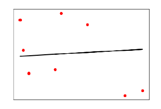
Look at the below diagram to understand why we need polynomial regression for non-linear data.
The above diagram shows the simple linear model hardly fits the data points whereas the polynomial model fits most of the data points.
Equation of Polynomial Regression Model
In machine learning, the general formula for polynomial regression of degree n is as follows −
y=w0+w1x+w2x2+w3x3+…+wnxn+ϵ
Where
y is the dependent variable (output).
x is the independent variable (input).
w0,w1,w2,…,wn are the coefficients (parameters) of the model.
n is the degree of the polynomial (the highest power of x).
ϵ is the error term or residual, representing the difference between the observed value and the model’s prediction.
For a quadratic (second-degree) polynomial regression, the formula would be:
y=w0+w1x+w2x2+ϵ
This would fit a parabolic curve to the data points.
How does Polynomial Regression Work?
In machine learning, the polynomial regression actually works in a similar way as linear regression works. It is modeled as multiple linear regression. The input feature is transformed into polynomial features of higher degrees (x2,x3,…,xn). These features are now treated as separate independent variables as in multiple linear regression. Now, a multiple linear regressor is trained on these transformed polynomial features.
The polynomial regression is a special case of multiple linear regression but there is a difference that multiple linear regression assumes linearity of input features. Here, in polynomial regression, the transformed polynomial features are dependent on the original input feature.
Implementation of Polynomial Regression using Python
Let’s implement polynomial regression using Python. We will use a well known machine learning Python library, Scikit-learn for building a regression model.
Step 1: Data Preparation
In machine learning model building, the data preparation is very important step. Let’s prepare our data first. We will be using a dataset named ice_cream_selling_data.csv. It contains 49 data examples. It has an input feature/ independent variable (Temperature (C)) and target feature/ dependent variable (Ice Cream Sales (units)).
The following table represents the data in ice_cream_selling_data.csv file.
ice_cream_selling_data.csv
Temperature (C)
Ice Cream Sales (units)
-4.662262677
41.84298632
-4.316559447
34.66111954
-4.213984765
39.38300088
-3.949661089
37.53984488
-3.578553716
32.28453119
-3.455711698
30.00113848
-3.108440121
22.63540128
-3.081303324
25.36502221
-2.672460827
19.22697005
-2.652286793
20.27967918
-2.651498033
13.2758285
-2.288263998
18.12399121
-2.11186969
11.21829447
-1.818937609
10.01286785
-1.66034773
12.61518115
-1.326378983
10.95773134
-1.173123268
6.68912264
-0.773330043
9.392968661
-0.673752802
5.210162615
-0.149634867
4.673642541
-0.036156498
0.328625517
-0.033895286
0.897603187
0.008607699
3.165600008
0.149244574
1.931416029
0.688780908
2.576782245
0.693598873
4.625689458
0.874905029
0.789973651
1.024180814
2.313806358
1.240711619
1.292360811
1.359812674
0.953115312
1.740000012
3.782570136
1.850551926
4.857987801
1.999310369
8.943823209
2.075100597
8.170734936
2.31859124
7.412094028
2.471945997
10.33663062
2.784836463
15.99661997
2.831760211
12.56823739
2.959932091
21.34291574
3.020874314
20.11441346
3.211366144
22.8394055
3.270044068
16.98327874
3.316072519
25.14208223
3.335932412
26.10474041
3.610778478
28.91218793
3.704057438
17.84395652
4.130867961
34.53074274
4.133533788
27.69838335
4.899031514
41.51482194
Note − Create a CSV file with the above data and save it as ice_cream_selling_data.csv.
Import Python libraries and packages for data preparation
Let’s first import libraries and packages required in the data preparation step. We use Python pandas for reading CSV files. We use NumPy to convert the pandas data frame to NumPy array. Input and output features are NumPy arrays. We use preprocessing package from the Scikit-learn library for preprocessing related tasks such as transforming input feature to polynomial features.
import numpy as np
import pandas as pd
import matplotlib.pyplot as plt
from sklearn.preprocessing import PolynomialFeatures
Load the dataset
Load the ice_cream_selling_data.csv as a pandas dataframe. Learn more about data loading here.
data = pd.read_csv('/ice_cream_selling_data.csv')
data.head()
Let’s create independent variable (X) and the dependent variable (y).
X = data.iloc[:,0].values.reshape(-1,1)
y = data.iloc[:,1].values
Visualize the original datapoints
Let’s visualize the original data points to get some insight.
# Visualize the original data points
plt.scatter(X, y, color="green")
plt.title("Original Data")
plt.xlabel("Temperature (C)")
plt.ylabel("Ice Cream Sales (units)")
plt.show()
Output
The above graph shows a parabolic curve (polynomial with degree 2) that will fit the datapoints.
So the relationship between the dependent variable (“Ice Cream Sales (units)”) and independent variable (“Temperature (C)”) can be modeled using polynomial regression of degree 2.
Create a polynomial features object
Now, let’s create a polynomial feature object with degree 2. We will use PolynomialFeatures class from sklearn.preprocessing module to create the feature object.
degree =2# Degree of the polynomial
poly_features = PolynomialFeatures(degree=degree)
Let’s now transform the input data to include polynomial features
X_poly = poly_features.fit_transform(X)
Here X_poly is transformed polynomial features of original input features (X). The transformed data is of (49, 3) shape.
Step 2: Model Training
We have created polynomial features. Now, let’s build out the model. We use LinearRegression class from sklearn.linear_model module. As we already discussed, Polynomial regression is a special type of linear regression.
Let’s create a linear regression object lr_model and train (fit) the model with data.
from sklearn.linear_model import LinearRegression
lr_model = LinearRegression()#Now, fit the model (linear regression object) on the data
lr_model.fit(X_poly, y)
So far, we have trained our regression model lr_model
Step 3: Model Prediction and Testing
Now, we can use our model to predict the output. Before going to predict for new data, let’s predict for the existing data.
You can compare the predicted values with actual values.
Step 4: Evaluating Model Performance
To evaluate the model performance, the best metric is the R-squared score (Coefficient of determination). It measures the proportion of the variance in the dependent variable that is predictable from the independent variables.
from sklearn.metrics import r2_score

# get the predicted values for test dat
y_pred = lr_model.predict(X_poly)
r2 = r2_score(y, y_pred)print(r2)
Outout
0.9321137090423877
The r2_score is the most common metric used to evaluate a regression model. The high score indicates a better fit of the model with data. 1 represent perfect fit and 0 represents no relation between the predicted values and actual values.
Result Explanation − You can examine the above metrics. Our model shows an R-squared score of around 0.932, which means that approximately 93% of data points are scattered around the fitted regression curve. Another interpretation is that 93% of the variation in the output variables is explained by the input variables.
Step 5: Visualize the polynomial regression results
Let’s visualize the regression results for better understanding. We use the pyplot module from the Matplotlib library to plot the graph.
import matplotlib.pyplot as plt

# Visualize the polynomial regression results
plt.scatter(X, y, color="green")
plt.plot(X, y_pred, color='red', label=f'Polynomial Regression (degree={degree})')
plt.xlabel("Temperature (C)")
plt.ylabel("Ice Cream Sales (units)")
plt.legend()
plt.title('Polynomial Regression')
plt.show()
Output
The above graph shows that the polynomial regression with degree 2 fits well with the original data. The polynomial curve (parabola), in red color, represents the best-fit regression curve. This regression curve is used to predict the value. The graph also shows that the predicted values are close to the actual values.
Step 5: Model Prediction for New Data
Up to now, we have predicted the values in the dataset. Let’s use our regression model to predict new, unseen data.
Let’s take the Temperature (C) as 1.9929C and predict the units of Ice Cream Sales.
# Predict a new value
X_new = np.array([[1.9929]])# Example value to predict
X_new_poly = poly_features.transform(X_new)
y_new_pred = lr_model.predict(X_new_poly)print(y_new_pred)
Output
[8.57450466]
The above result shows that the predicted value of Ice cream sales is 8.57450466.
Multiple linear regression in machine learning is a supervised algorithm that models the relationship between a dependent variable and multiple independent variables. This relationship is used to predict the outcome of the dependent variable.
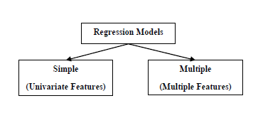
Multiple linear regression is a type of linear regression in machine learning. There are mainly two types of linear regression algorithms −
simple linear regression − it deals with two features (one dependent variable and one independent variable).
multiple linear regression − deals with more than two features (one dependent variable and more than one independent variables).
Let’s discuss multiple linear regression in detail −
What is Multiple Linear Regression?
In machine learning, multiple linear regression (MLR) is a statistical technique that is used to predict the outcome of a dependent variable based on the values of multiple independent variables. The multiple linear regression algorithm is trained on data to learn a relationship (known as a regression line) that best fits the data. This relation describes how various factors affect the result. This relation is used to forecast the value of dependent variable based on the values of independent variables.
In linear regression (simple and multiple), the dependent variable is continuous (numeric value) and independent variables can be continuous or discreet (numeric value). Independent variables can also be categorical (gender, occupation), but they need to be converted to numerical values first.
Multiple linear regression is basically the extension of simple linear regression that predicts a response using two or more features. Mathematically we can represent the multiple linear regression as follows −
Consider a dataset having n observations, p features i.e. independent variables and y as one response i.e. dependent variable the regression line for p features can be calculated as follows −
h(xi)=w0+w1xi1+w2xi2+⋅⋅⋅+wpxip
Here, h(xi) is the predicted response value and w0,w1,w2….wp are the regression coefficients.
Multiple Linear Regression models always includes the errors in the data known as residual error which changes the calculation as follows −
yi=w0+w1xi1+w2xi2+⋅⋅⋅+wpxip+ei
We can also write the above equation as follows −
yi=h(xi)+eiorei=yi−h(xi)
Assumptions of Multiple Linear Regression
The following are some assumptions about the dataset that are made by the multiple linear regression model −
1. Linearity
The relationship between the dependent variable (target) and independent (predictor) variables is linear.
2. Independence
Each observation is independent of others. The value of the dependent variable for one observation is independent of the value of another.
3. Homoscedasticity
For all observations, the variance of the residual errors is similar across the value of each independent variable.
4. Normality of Errors
The residuals (errors) are normally distributed. The residuals are differences between the actual and predicted values.
5. No Multicollinearity
The independent variables are not highly correlated with each other. Linear regression models assume that there is very little or no multi-collinearity in the data.
6. No Autocorrelation
There is no correlation between residuals. This ensures that the residuals (errors) are independent of each other.
7. Fixed Independent Variables
The values of independent variables are fixed in all repeated samples.
Violations of these assumptions can lead to biased or inefficient estimates. It is essential to validate these assumptions to ensure model accuracy.
Implementing Multiple Linear Regression in Python
To implement multiple linear regression in Python using Scikit-Learn, we can use the same LinearRegression class as in simple linear regression, but this time we need to provide multiple independent variables as input.
Step 1: Data Preparation
We use the dataset named data.csv with 50 examples. It contains four predictor (independent) variables and a target (dependent) variable. The following table represents the data in data.csv file.
data.csv
R&D Spend
Administration
Marketing Spend
State
Profit
165349.2
136897.8
471784.1
New York
192261.8
162597.7
151377.6
443898.5
California
191792.1
153441.5
101145.6
407934.5
Florida
191050.4
144372.4
118671.9
383199.6
New York
182902
142107.3
91391.77
366168.4
Florida
166187.9
131876.9
99814.71
362861.4
New York
156991.1
134615.5
147198.9
127716.8
California
156122.5
130298.1
145530.1
323876.7
Florida
155752.6
120542.5
148719
311613.3
New York
152211.8
123334.9
108679.2
304981.6
California
149760
101913.1
110594.1
229161
Florida
146122
100672
91790.61
249744.6
California
144259.4
93863.75
127320.4
249839.4
Florida
141585.5
91992.39
135495.1
252664.9
California
134307.4
119943.2
156547.4
256512.9
Florida
132602.7
114523.6
122616.8
261776.2
New York
129917
78013.11
121597.6
264346.1
California
126992.9
94657.16
145077.6
282574.3
New York
125370.4
91749.16
114175.8
294919.6
Florida
124266.9
86419.7
153514.1
0
New York
122776.9
76253.86
113867.3
298664.5
California
118474
78389.47
153773.4
299737.3
New York
111313
73994.56
122782.8
303319.3
Florida
110352.3
67532.53
105751
304768.7
Florida
108734
77044.01
99281.34
140574.8
New York
108552
64664.71
139553.2
137962.6
California
107404.3
75328.87
144136
134050.1
Florida
105733.5
72107.6
127864.6
353183.8
New York
105008.3
66051.52
182645.6
118148.2
Florida
103282.4
65605.48
153032.1
107138.4
New York
101004.6
61994.48
115641.3
91131.24
Florida
99937.59
61136.38
152701.9
88218.23
New York
97483.56
63408.86
129219.6
46085.25
California
97427.84
55493.95
103057.5
214634.8
Florida
96778.92
46426.07
157693.9
210797.7
California
96712.8
46014.02
85047.44
205517.6
New York
96479.51
28663.76
127056.2
201126.8
Florida
90708.19
44069.95
51283.14
197029.4
California
89949.14
20229.59
65947.93
185265.1
New York
81229.06
38558.51
82982.09
174999.3
California
81005.76
28754.33
118546.1
172795.7
California
78239.91
27892.92
84710.77
164470.7
Florida
77798.83
23640.93
96189.63
148001.1
California
71498.49
15505.73
127382.3
35534.17
New York
69758.98
22177.74
154806.1
28334.72
California
65200.33
1000.23
124153
1903.93
New York
64926.08
1315.46
115816.2
297114.5
Florida
49490.75
0
135426.9
0
California
42559.73
542.05
51743.15
0
New York
35673.41
0
116983.8
45173.06
California
14681.4
You can create a CSV file and store the above data points in it.
We have our dataset as data.csv file. We will use it to understand the implementation of the multiple linear regression in Python.
We need to import libraries before loading the dataset.
# import librariesimport numpy as np
import matplotlib.pyplot as plt
import pandas as pd
Load the dataset
We load our dataset as a Pandas Data frame named <string>dataset. Now let’s create a list of independent values (predictors) and put them in a variable called X.</string>
The independent values are ‘R&D Spend’, ‘Administration’, ‘Marketing Spend’. We are not using the independent variable ‘State’ for sake of simplicity.
We put the dependent variable values to a variable y.
# load dataset
dataset = pd.read_csv('data.csv')
X = dataset[['R&D Spend','Administration','Marketing Spend']]
y = dataset['Profit']
Let’s check first five examples (rows) of input features (X) and target (y) −
Now, we split the dataset into a training set and a test set. Both the X(independent values) and y (dependent values) are divided into two sets – training and test. We will use 20% for the test set. In such a way out of 50 feature vectors (observations/ examples), there will be 40 feature vectors in training set and 10 feature vectors in test set.
# Split the dataset into training and test sets from sklearn.model_selection import train_test_split
X_train, X_test, y_train, y_test = train_test_split(X, y, test_size =0.2)
Here X_train and X_test represent input features in training set and test set, where y_train and y_test represent target values (output) in traning and test set.
Step 2: Model Training
The next step is to fit our model with training data. We will use linear_model class from sklearn module. We use the Linear Regression() method of linear_model class to create a linear regression object, here we name it as regressor.
# Fit Multiple Linear Regression to the Training setfrom sklearn.linear_model import LinearRegression
regressor = LinearRegression()
regressor.fit(X_train, y_train)
The regressor object has fit() method. The fit() method is used to fit the linear regression object, regressor to the training data. The model learns the relation between the predictor variable (X_train), and the target variable (y_train).
Step 3: Model Testing
Now our model is ready to use for prediction. Let’s test our regressor model on test data.
We use predict() method to predict the results for the test set. It takes input features (X_test) and return the redicted values.
You can compare the actual values and predicted values.
Step 4: Model Evaluation
We now evaluate our model to check how accurate it is. We will use mean square error (MSE), root mean square error (RMSE), mean absolute error (MAE), and R2-score (Coefficient of determination).
from sklearn.metrics import mean_squared_error, root_mean_squared_error, mean_absolute_error, r2_score
# Assuming you have your true y values (y_test) and predicted y values (y_pred)
mse = mean_squared_error(y_test, y_pred)
rmse = root_mean_squared_error(y_test, y_pred)
mae = mean_absolute_error(y_test, y_pred)
r2 = r2_score(y_test, y_pred)print("Mean Squared Error (MSE):", mse)print("Root Mean Squared Error (RMSE):", rmse)print("Mean Absolute Error (MAE):", mae)print("R-squared (R2):", r2)
Output
Mean Squared Error (MSE): 72684687.6336162
Root Mean Squared Error (RMSE): 8525.531516193943
Mean Absolute Error (MAE): 6425.118502810154
R-squared (R2): 0.9588459519573707
You can examine the above metrics. Our model shows an R-squared score of around 0.96, which means that 96% of data points are scattered around the fitted regression line. Another interpretation is that 96% of the variation in the output variables is explained by the input variables.
Step 5: Model Prediction for New Data
Let’s use our regressor model to predict profit values based on R&D Spend, Administration and Marketing Spend.
Predicting sales, customer churn, and marketing campaign effectiveness.
Real Estate
Predicting house prices based on factors like size, location, and number of bedrooms.
Healthcare
Predicting patient outcomes, analyzing the impact of treatments, and identifying risk factors for diseases.
Economics
Forecasting economic growth, analyzing the impact of policies, and predicting inflation rates.
Social Sciences
Modeling social phenomena, predicting election outcomes, and understanding human behavior.
Challenges of Multiple Linear Regression
The following are some common challenges faced by multiple linear regression in machine learning −
Challenge
Description
Multicollinearity
High correlation between independent variables, leading to unstable model coefficients and difficulty in interpreting the impact of individual variables.
Overfitting
The model fits the training data too closely, leading to poor performance on new, unseen data.
Underfitting
The model fails to capture the underlying patterns in the data, resulting in poor performance on both training and test data.
Non-linearity
Multiple linear regression assumes a linear relationship between the independent and dependent variables. Non-linear relationships can lead to inaccurate predictions.
Outliers
Outliers can significantly impact the model’s performance, especially in small datasets.
Missing Data
Missing data can lead to biased and inaccurate results.
Difference Between Simple and Multiple Linear Regression
The following table highlights the major differences between simple and multiple linear regression −
Feature
Simple Linear Regression
Multiple Linear Regression
Independent Variables
One
Two or more
Model Equation
y = w1x + w0
y=w0+w1x1+w2x2+ … +wpxp
Complexity
Less complex
More complex due to multiple variables
Real-world Applications
Predicting house prices based on square footage, predicting sales based on advertising expenditure
Predicting sales based on advertising expenditure, price, and competitor activity, predicting student performance based on study hours, attendance, and IQ
Model Interpretation
Easier to interpret coefficients
More complex to interpret due to multiple variables
Simple linear regression is a statistical and supervised learning method in which a single independent variable (also known as a predictor variable) is used to predict the dependent variable. In other words, it models the linear relationship between the dependent variable and a single independent variable.
Simple linear regression in machine learning is a type of linear regression. When the linear regression algorithm deals with a single independent variable, it is known as simple linear regression. When there is more than one independent variable (feature variables), it is known as multiple linear regression.
Independent Variable
The feature inputs in the dataset are termed as the independent variables. There is only a single independent variable in simple linear regression. An independent variable is also known as a predictor variable as it is used to predict the target value. It is plotted on a horizontal axis.
Dependent Variable
The target value in the dataset is termed as the dependent variable. It is also known as a response variable or predicted variable. It is plotted on a vertical axis.
Line of Regression
In simple linear regression, a line of regression is a straight line that best fits the data points and is used to show the relationship between a dependent variable and an independent variable.
Graphical Representation
The following graph depicts the simple linear regression model −
In the above image, the straight line represents the simple linear regression line where Ŷ is the predicted value, and Y is dependent variable (target) and X is independent variable (input).
Simple Linear Regression Model
A simple linear regression model in machine learning can be represented as the following mathematical equation −
Y=w0+w1X+ϵ
Where
Y is the dependent variable (target).
X is the independent variable (feature).
w0 is the y-intercept of the line.
w1 is the slope of the line, representing the effect of X on Y.
ε is the error term, capturing the variability in Y not explained by X.
How Simple Linear Regression Works?
The main of simple linear regression is to find the best fit line (a straight line) through the data points that minimizes the difference between the actual values and predicted values.
Defining Hypothesis Function
In simple linear regression, the hypothesis is that there is a linear relation between the dependent variable (output/ target) and the independent variable (input). This linear relation can be represented using a linear equation −
Ŷ =w0+w1X
With different values of parameters w0 and w1 there are multiple linear equations (straight lines). The set of all such linear equations (all straight lines) is termed hypothesis space.
Now, the main aim of the simple linear regression model is to find the best-fit line in Hypothesis space (set of all straight lines).
Finding the Best Fit Line
Now the task is to find the best fit line (line of regression). To do this, we define a cost function or loss function that measure the the difference between the actual values and predicted values.
To find the best fit line, the simple linear regression model initializes (with default values) the parameters of the regression line. This regression line (with initialized parameters) is used to find the predicted values for the given input values.
Loss Function for Simple Linear Regression
Now using the input and predicted values, we compute the loss function. The loss function is used to find the optimal values of the parameters.
The loss function finds the difference between the input value and predicted value. There are different loss functions such as mean squared error (MSE), mean absolute error (MEA), R-squared, etc. used in simple linear regression. The most commonly used loss function is mean squared error.
The loss function for simple linear regression in terms of mean squared error is as follows −
J(w0,w1)=12n∑i=1n(Yi−Ŷ i)2
Optimization
The optimal values of parameters are those values that minimize the cost function. Finding the optimal values is an iterative process in which the parameters are updated iteratively.
There are many optimization techniques applied in simple linear regression. Gradient Descent is a simple and most common optimization technique used in simple linear regression.
A linear equation with optimal parameter values is the best fit line(regression line) and it is the final solution for a simple linear regression problem. This line is used to predict new and unseen data.
Assumptions of Simple Linear Regression
There are some assumptions about the dataset that are made by the simple linear regression model. The following are some assumptions −
Linearity − This assumption assumes that the relationship between the dependent and independent variables is linear. That means the dependent variable changes linearly as the independent variable changes. A scatter plot will show the linearity in the dataset.
Homoskedasticity − For all observations, the variance of the residuals is the same. This assumption relates to the squared residuals.
Independence − The examples (observations or X and Y pairs) are independent. There is no collinearity in data so the residuals will not be correlated. To check this, we example the scatter plot of residuals vs. fits.
Normality − Model Residuals are normally distributed. Residuals are the differences between the actual and predicted values. To check for the normality, we examine the histogram of residuals. The histogram should be approximately normally distributed.
Implementation of Simple Linear Regression Algorithm using Python
To implement the simple linear regression algorithm, we are taking a dataset with two variables: YearsExperience (independent variable) and Salary (dependent variable).
Here, we are using the following dataset. The dataset contains 30 examples of data points. You can create a CSV file and store these data points in it.
Salary_Data.csv
Years of Experience
Salary
1.1
39343
1.3
46205
1.5
37731
2
43525
2.2
39891
2.9
56642
3
60150
3.2
54445
3.2
64445
3.7
57189
3.9
63218
4
55794
4
56957
4.1
57081
4.5
61111
4.9
67938
5.1
66029
5.3
83088
5.9
81363
6
93940
6.8
91738
7.1
98273
7.9
101302
8.2
113812
8.7
109431
9
105582
9.5
116969
9.6
112635
10.3
122391
10.5
121872
What is the purpose of this implementation?
The purpose of building this simple linear regression model is to determine which line best represents the relationship between the two variables.
The following are the steps to implement the simple linear regression model in Python −
Step 1: Data Preparation
Data preparation or pre-processing is the initial step. We have our dataset as a CSV file named “Salary_Data.csv,” as discussed above.
We need to import python libraries prior to importing the dataset and building the simple linear regression model.
import numpy as np
import matplotlib.pyplot as plt
import pandas as pd
Load the dataset
dataset = pd.read_csv('Salary_Data.csv')
The dependent variable (X) and independent variable (Y) must then be extracted from the provided dataset. Years of experience (YearsExperience) is the independent variable, and Salary is the dependent variable.
X = dataset.iloc[:,:-1].values
y = dataset.iloc[:,-1].values
Let’s check the first five examples of the dataset.
plt.scatter(X, y, color="green")
plt.title("Salary vs Experience")
plt.xlabel("Years of Experience")
plt.ylabel("Salary (INR)")
plt.show()
Output
The above graph shows that the dependent and independent variables are linearly dependent. So we can apply the simple linear regression on the dataset to find the best relation between these variables.
Split the dataset into training and testing sets
The training set and test set will then be divided into two groups. We will use 80% observations for the training set and 20% observations for the test set out of the total 30 observations we have. So there will be 24 observation in training set and 6 observation in test set. We divide our dataset into training and test sets so that we can use one set to train and the other to test our model.
# Split the dataset into training and testing setsfrom sklearn.model_selection import train_test_split
X_train, X_test, y_train, y_test = train_test_split(X, y, test_size =0.2)
Here, X_train represents the input feature of the training data and y_train represents the output variable (target variable).
Step 2: Model Training (Fitting the Simple Linear Regression to Training Set)
The next step is fitting our model with the training dataset. We will use scikit-learn’s LinearRegression class to train a simple linear regression model on the training data. The code for this is as follows −
from sklearn.linear_model import LinearRegression

# Create a linear regression object
regressor= LinearRegression()
regressor.fit(X_train, y_train)
The fit() method is used to fit the linear regression object (regressor) to the training data. The model learns the relation between the predictor variable (X_train), and the target variable (y_train).
Step 3: Model Testing
Once the model is trained, we can use it to make predictions on the test data. The code for this is as follows −
We need to evaluate the performance of the model to determine its accuracy. We will use the mean squared error (MSE), root mse (RMSE), mean average error (MAE), and the coefficient of determination (R^2) as evaluation metrics. The code for this is as follows −
from sklearn.metrics import mean_squared_error
from sklearn.metrics import mean_absolute_error
from sklearn.metrics import r2_score

# get the predicted values for test dat
y_pred = regressor.predict(X_test)
mse = mean_squared_error(y_test, y_pred)print("mse", mse)
rmse = mean_squared_error(y_test, y_pred, squared=False)print("rsme", rmse)
mae = mean_absolute_error(y_test, y_pred)print("mae", mae)
r2 = r2_score(y_test, y_pred)print("r2", r2)
Here, y_test represents the actual output variable of the test data.
Step 5: Visualize Training Set Results (with Regression Line)
Now, let’s visualize the results on the training set and the regression line.
We use the scatter plot to plot the actual values (input and target values) in the training set. We also plot a straight line (regression line) for actual values (input) and predicted values of the training set.
y_pred = regressor.predict(X_train)
plt.scatter(X_train, y_train, color="green", label="training data points (actual)")
plt.scatter(X_train, y_pred, color="blue",label="training data points (predicted)")
plt.plot(X_train, y_pred, color="red")
plt.title("Salary vs Experience (Training Dataset)")
plt.xlabel("Years of Experience")
plt.ylabel("Salary(In Rupees)")
plt.legend()
plt.show()
Output
The above graph shows the line of regression (straight line in red color), actual values (in green color), and predicted values (in blue color) for the training set.
Step 6: Visualize the Test Set Results (with Regression Line)
Now, let’s visualize the results on the test set and the regression line.
We use the scatter plot to plot the actual values (input and target values) in the test set. We also plot a straight line (regression line) for actual values (input) and predicted values of the test set.
y_pred = regressor.predict(X_test)
plt.scatter(X_test, y_test, color="green", label="test data points (actual)")
plt.scatter(X_test, y_pred, color="blue",label="test data points (predicted)")
plt.plot(X_test, y_pred, color="red")
plt.title("Salary vs Experience (Test Dataset)")
plt.xlabel("Years of Experience")
plt.ylabel("Salary(In Rupees)")
plt.legend()
plt.show()
Output
The above graph shows the line of regression (straight line in red color), actual values (in green color), and predicted values (in blue color) for the test set.
Linear regression in machine learning is defined as a statistical model that analyzes the linear relationship between a dependent variable and a given set of independent variables. The linear relationship between variables means that when the value of one or more independent variables will change (increase or decrease), the value of the dependent variable will also change accordingly (increase or decrease).
In machine learning, linear regression is used for predicting continuous numeric values based on learned linear relation for new and unseen data. It is used in predictive modeling, financial forecasting, risk assessment, etc.
In this chapter, we will discuss the following topics in detail −
What is Linear Regression?
Types of Linear Regression
How Does Linear Regression Work?
Hypothesis Function For Linear Regression
Finding the Best Fit Line
Loss Function For Linear Regression
Gradient Descent for Optimization
Assumptions of Linear Regression
Evaluation Metrics for Linear Regression
Applications of Linear Regression
Advantages of Linear Regression
Common Challenges with Linear Regression
What is Linear Regression?
Linear regression is a statistical technique that estimates the linear relationship between a dependent and one or more independent variables. In machine learning, linear regression is implemented as a supervised learning approach. In machine learning, labeled datasets contain input data (features) and output labels (target values). For linear regression in machine learning, we represent features as independent variables and target values as the dependent variable.
For the simplicity, take the following data (Single feature and single target)
Square Feet (X)
House Price (Y)
1300
240
1500
320
1700
330
1830
295
1550
256
2350
409
1450
319
In the above data, the target House Price is the dependent variable represented by X, and the feature, Square Feet, is the independent variable represented by Y. The input features (X) are used to predict the target label (Y). So, the independent variables are also known as predictor variables, and the dependent variable is known as the response variable.
So lets define linear regression in machine learning as follows:
In machine learning, linear regression uses a linear equation to model the relationship between a dependent variable (Y) and one or more independent variables (Y).
The main goal of the linear regression model is to find the best-fitting straight line (often called a regression line) through a set of data points.
Line of Regression
A straight line that shows a relation between the dependent variable and independent variables is known as the line of regression or regression line.
Furthermore, the linear relationship can be positive or negative in nature as explained below −
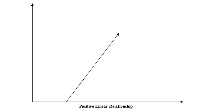
1. Positive Linear Relationship
A linear relationship will be called positive if both independent and dependent variable increases. It can be understood with the help of the following graph −
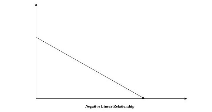
2. Negative Linear Relationship
A linear relationship will be called positive if the independent increases and the dependent variable decreases. It can be understood with the help of the following graph −
Linear regression is of two types, “simple linear regression” and “multiple linear regression”, which we are going to discuss in the next two chapters of this tutorial.
Types of Linear Regression
Linear regression is of the following two types −
Simple Linear Regression
Multiple Linear Regression
1. Simple Linear Regression
Simple linear regression is a type of regression analysis in which a single independent variable (also known as a predictor variable) is used to predict the dependent variable. In other words, it models the linear relationship between the dependent variable and a single independent variable.
In the above image, the straight line represents the simple linear regression line where Ŷ is the predicted value, and X is the input value.
Mathematically, the relationship can be modeled as a linear equation −
Y=w0+w1X+ϵ
Where
Y is the dependent variable (target).
X is the independent variable (feature).
w0 is the y-intercept of the line.
w1 is the slope of the line, representing the effect of X on Y.
ε is the error term, capturing the variability in Y not explained by X.
2. Multiple Linear Regression
Multiple linear regression is basically the extension of simple linear regression that predicts a response using two or more features.
When dealing with more than one independent variable, we extend simple linear regression to multiple linear regression. The model is expressed as:
Multiple linear regression extends the concept of simple linear regression to multiple independent variables. The model is expressed as:
Y=w0+w1X1+w2X2+⋯+wpXp+ϵ
Where
X1, X2, …, Xp are the independent variables (features).
w0, w1, …, wp are the coefficients for these variables.
ε is the error term.
How Does Linear Regression Work?
The main goal of linear regression is to find the best-fit line through a set of data points that minimizes the difference between the actual values and predicted values. So it is done? This is done by estimating the parameters w0, w1 etc.
The working of linear regression in machine learning can be broken down into many steps as follows −
Hypothesis − We assume that there is a linear relation between input and output.
Cost Function − Define a loss or cost function. The cost function quantifies the model’s prediction error. The cost function takes the model’s predicted values and actual values and returns a single scaler value that represents the cost of the model’s prediction.
Optimization − Optimize (minimize) the model’s cost function by updating the model’s parameters.
It continues updating the model’s parameters until the cost or error of the model’s prediction is optimized (minimized).
Let’s discuss the above three steps in more detail −
Hypothesis Function For Linear Regression
In linear regression problems, we assume that there is a linear relationship between input features (X) and predicted value (Ŷ).
The hypothesis function returns the predicted value for a given input value. Generally we represent a hypothesis by hw(X) and it is equal to Ŷ.
Hypothesis function for simple linear regression −
Ŷ =w0+w1X
Hypothesis function for multiple linear regression −
Ŷ =w0+w1X1+w2X2+⋯+wpXp
For different values of parameters (weights), we can find many regression lines. The main goal is to find the best-fit lines. Let’s discuss it as below −
Finding the Best Fit Line
We discussed above that different set of parameters will provide different regression lines. However, each regression line does not represent the optimal relation between the input and output values. The main goal is to find the best-fit line.
A regression line is said to be the best fit if the error between actual and predicted values is minimal.
Below image shows a regression line with error (ε) at input data point X. The error is calculated for all data points and our goal is to minimize the average error/ loss. We can use different types of loss functions such as mean square error (MSE), mean average error (MAE), L1 loss, L2 Loss, etc.
So, how can we minimize the error between the actual and predicted values? Let’s discuss the important concept, which is cost function or loss function.
Loss Function for Linear Regression
The error between actual and predicted values can be quantified using a loss function of the cost function. The cost function takes the model’s predicted values and actual values and returns a single scaler value that represents the cost of the model’s prediction. Our main goal is to minimize the cost function.
The most commonly used cost function is the mean squared error function.
J(w0,w1)=12n∑i=1n(Yi−Ŷ i)2
Where,
n is the number of data points.
Yi is the observed value for the i-th data point.
Ŷ i=w0+w1Xi is the predicted value for the i-th data point.
Gradient Descent for Optimization
Now we have defined our loss function. The next step is to minimize it and find the optimized values of the parameters or weights. This process of finding optimal values of parameters such that the loss or error is minimal is known as model optimization.
Gradient Descent is one of the most used optimization techniques for linear regression.
To find the optimal values of parameters, gradient descent is often used, especially in cases with large datasets. Gradient descent iteratively adjusts the parameters in the direction of the steepest descent of the cost function.
The parameter updates are given by
w0=w0−α∂J∂w0
w1=w1−α∂J∂w1
Where α is the learning rate, and the partial derivatives are:
∂J∂w0=−1n∑i=1n(Yi−Ŷ i)
∂J∂w1=−1n∑i=1n(Yi−Ŷ i)Xi
These gradients are used to update the parameters until convergence is reached (i.e., when the changes in w0 and w1 become negligible).
Assumptions of Linear Regression
The following are some assumptions about the dataset that are made by the Linear Regression model −
Multi-collinearity − Linear regression model assumes that there is very little or no multi-collinearity in the data. Basically, multi-collinearity occurs when the independent variables or features have a dependency on them.
Auto-correlation − Another assumption the Linear regression model assumes is that there is very little or no auto-correlation in the data. Basically, auto-correlation occurs when there is dependency between residual errors.
Relationship between variables − Linear regression model assumes that the relationship between response and feature variables must be linear.
Violations of these assumptions can lead to biased or inefficient estimates. It is essential to validate these assumptions to ensure model accuracy.
Evaluation Metrics for Linear Regression
To assess the performance of a linear regression model, several evaluation metrics are used −
R-squared (R2) − It measures the proportion of the variance in the dependent variable that is predictable from the independent variables.
R2=1−∑(yi−ŷ i)2∑(yi−y¯)2
Mean Squared Error (MSE) − It measures an average of the sum of the squared difference between the predicted values and the actual values.
MSE=1n∑i=1n(yi−ŷ i)2
Root Mean Squared Error (RMSE) − It measures the square root of the MSE.
RMSE=MSE‾‾‾‾‾√
Mean Absolute Error (MAE) − It measures the average of the sum of the absolute values of the difference between the predicted values and the actual values.
MAE=1n∑i=1n|yi−ŷ i|
Applications of Linear Regression
1. Predictive Modeling
Linear regression is widely used for predictive modeling. For instance, in real estate, predicting house prices based on features such as size, location, and number of bedrooms can help buyers, sellers, and real estate agents make informed decisions.
2. Feature Selection
In multiple linear regression, analyzing the coefficients can help in feature selection. Features with small or zero coefficients might be considered less important and can be dropped to simplify the model.
3. Financial Forecasting
In finance, linear regression models predict stock prices, economic indicators, and market trends. Accurate forecasts can guide investment strategies and financial planning.
4. Risk Management
Linear regression helps in risk assessment by modeling the relationship between risk factors and financial metrics. For example, in insurance, it can model the relationship between policyholder characteristics and claim amounts.
Advantages of Linear Regression
Interpretability − Linear regression is easy to understand, which is useful when explaining how a model makes decisions.
Speed − Linear regression is faster to train than many other machine learning algorithms.
Predictive analytics − Linear regression is a fundamental building block for predictive analytics.
Linear relationships − Linear regression is a powerful statistical method for finding linear relationships between variables.
Simplicity − Linear regression is simple to implement and interpret.
Efficiency − Linear regression is efficient to compute.
Common Challenges with Linear Regression
1. Overfitting
Overfitting occurs when the regression model performs well on training data but lacks generalization on test data. Overfitting leads to poor prediction on new, unseen data.
2. Multicollinearity
When the dependent variables (predictor or feature variables) correlate, the situation is known as mutilcolinearty. In this, the estimates of the parameters (coefficients) can be unstable.
3. Outliers and Their Impact
Outliers can cause the regression line to be a poor fit for the majority of data points.
Polynomial Regression: An Alternate to Linear Regression
Polynomial Linear Regression is a type of regression analysis in which the relationship between the independent variable and the dependent variable is modeled as an n-th degree polynomial function. Polynomial regression allows for a more complex relationship between the variables to be captured beyond the linear relationship in Simple and Multiple Linear Regression.
In machine learning, regression analysis is a statistical technique that predicts continuous numeric values based on the relationship between independent and dependent variables. The main goal of regression analysis is to plot a line or curve that best fit the data and to estimate how one variable affects another.
Regression analysis is a fundamental concept in machine learning and it is used in many applications such as forecasting, predictive analytics, etc.
In machine learning, regression is a type of supervised learning. The key objective of regression-based tasks is to predict output labels or responses, which are continuous numeric values, for the given input data. The output will be based on what the model has learned in the training phase.
Regression models use the input data features (independent variables) and their corresponding continuous numeric output values (dependent or outcome variables) to learn specific associations between inputs and corresponding outputs.
Terminologies Used In Regression Analysis
Let us understand some basic terminologies used in regression analysis before going into further detail. The following are some important terminologies −
Independent Variables − These variables are used to predict the value of the dependent variable. These are also called predictors. In dataset, these are represented as features.
Dependent Variables − These are the variables whose values we want to predict. These are the main factors in regression analysis. In dataset, these are represented as target variables
Regression line − It is a straight line or curve that a regressor plots to fit the data points best.
Overfitting and underfitting − Overfitting is when the regression model works well with the training dataset but not with the testing dataset. It’s also referred to as the problem of high variance. Underfitting is when the model doesn’t work well with training datasets. It’s also referred to as the problem of high bias.
Outliers − These are data points that don’t fit the pattern of the rest of the data. They are the extremely high or extremely low values in the data set.
Multicollinearity − multicollinearity occurs when independent variables (features) have dependency among them.
How Does Regression Work?
Regression in machine learning is a supervised learning. Basically, regression is a statistical technique that finds a relationship between dependent and independent variables. To implement regression in machine learning, a regression algorithm is trained with a labeled dataset. The dataset contains features (independent variables) and target values (dependent variable).
During the training phase, the regression algorithm learns the relation between independent variables (predictors) and dependent variables (target).
The regression models predict new values based on the learned relation between predictors and targets during the training.
Types of Regression in Machine Learning
Generally, the classification of regression methods is done based on the three metrics − the number of independent variables, type of dependent variables, and shape of the regression line.
There are numerous regression techniques used in machine learning. However, the following are commonly used types of regression −
Linear Regression
Logistic Regression
Polynomial Regression
Lasso Regression
Ridge Regression
Decision Tree Regression
Random Forest Regression
Support Vector Regression
Let’s discuss each type of regression in machine learning in detail.
1. Linear Regression
Linear regression is the most commonly used regression model in machine learning. It may be defined as the statistical model that analyzes the linear relationship between a dependent variable with a given set of independent variables. A linear relationship between variables means that when the value of one or more independent variables changes (increase or decrease), the value of the dependent variable will also change accordingly (increase or decrease).
Linear regression is further divided into two subcategories: simple linear regression and multiple linear regression (also known as multivariate linear regression).
In simple linear regression, a single independent variable (or predictor) is used to predict the dependent variable.
Mathematically, the simple linear regression can be represented as follows −
Y=mX+b
Where,
Y is the dependent variable we are trying to predict.
X is the dependent variable we are using to make predictions.
m is the slope of the regression line, which represents the effect X has on Y.
b is a constant known as the Y-intercept. If X=0, Y would be equal to b.
In multi-linear regression, multiple independent variables are used to predict the dependent variables.
We will learn linear regression in more detail in upcoming chapters.
2. Logistic Regression
Logistic regression is a popular machine learning algorithm used for predicting the probability of an event occurring.
Logistic regression is a generalized linear model where the target variable follows a Bernoulli distribution. Logistic regression uses a logistic function or logit function to learn a relationship between the independent variables (predictors) and dependent variables (target).
It maps the dependent variable as a sigmoid function of independent variables. The sigmoid function produces a probability between 0 and 1. The probability value is used to estimate the dependent variable’s value.
It is mostly used in binary classification problems, where the target variable is categorical with two classes. It models the probability of the target variable given the input features and predicts the class with the highest probability.
3. Polynomial Regression
Polynomial Linear Regression is a type of regression analysis in which the relationship between the independent variable and the dependent variable is modeled as an n-th degree polynomial function. Polynomial regression allows for a more complex relationship between the variables to be captured, beyond the linear relationship in Simple and Multiple Linear Regression.
Polynomial regression is one of the most widely used non-linear regressions. It is very useful because it can model non-linear relationships between predictors and targets, and also it is more sensitive to outliers.
4. Lasso Regression
Lasso regression is a regularization technique that uses a penalty to prevent overfitting and improve the accuracy of regression models. It performs L1 regularization. It modifies the loss function by adding the penalty (shrinkage quantity) equivalent to the summation of the absolute value of coefficients.
Lasso regression is often used to handle high dimensional and high correlation data.
5. Ridge Regression
Ridge regression is a statistical technique used in machine learning to prevent overfitting in linear regression models. It is used as a regularization technique that performs L2 regularization. It modifies the loss or cost function by adding the penalty (shrinkage quantity) equivalent to the square of the magnitude of coefficients.
Ridge regression helps to reduce model complexity and improve prediction accuracy. It is useful in developing many parameters with high weights. It is also well suited to datasets with more feature variables than a number of observations.
It also corrects the multicollinearity in regression analysis. Multicollinearity occurs when independent variables are dependent on each other.
6. Decision Tree Regression
Decision tree regression uses the decision tree algorithm to predict numerical values. The decision tree algorithm is a supervised machine learning algorithm that can be used for both classification and regression.
It is used to predict numerical values or continuous variables. It works by splitting the data into smaller subsets based on the values of the input features and assigning each subset a numerical value. So incrementally, it develops a decision tree
The tree fits local linear regressions that approximate a curve, and each leaf represents a numeric value. The algorithm tries to reduce the mean square error at each child node, which measures how much the predictions deviate from the original target.
The decision tree regression can be used in predicting stock prices or customer behavior etc.
7. Random Forest Regression
Random forest regression is a supervised machine learning algorithm that uses an ensemble of decision trees to predict continuous target variables. It uses a bagging technique that involves randomly selecting subsets of training data to build smaller decision trees. These smaller models are combined to form a random forest model that outputs a single prediction value.
The technique helps improve accuracy and reduce variance by combining the predictions from multiple decision trees.
8. Support Vector Regression
Support vector regression (SVR) is a machine learning algorithm that uses support vector machine to solve regression problems. It can learn non-linear relationships between the input data (feature variables) and output data (target values).
Support vector regression has many advantages. It can handle linear as well as non-linear relationships in datasets. It is resistant to outliers. It has high prediction accuracy.
Types of Regression Models
Regression models are of following two types −
Simple regression model − This is the most basic regression model in which predictions are formed from a single, univariate feature of the data.
Multiple regression model − As the name implies, in this regression model, the predictions are formed from multiple features of the data.
How to Select Best Regression Model?
You can consider factors like performance metrics, model complexity, interpretability, etc., to select the best regression model. Evaluate the model performance using metrics such as Mean Squared Error (MSE), Mean absolute error (MAE), R-squared, etc. Compare the performance of different models, such as linear regression, decision trees, random forests, etc., and choose a model that has the highest performance metrics, the lowest complexity, and the best interpretability.
Evaluation Metrics for Regression
Common evaluation/ performance metrics for regression models −
Mean Absolute error (MAE) − It is the average of the absolute difference between predicted values and true values.
Mean Squared error (MSE) − It is the average of the square of the difference between actual and estimated values.
Median Absolute error − It is the median value of the absolute difference between predicted values and true values.
Root mean square error (RMSE) − It is the square root value of the mean squared error (MSE).
R2 (coefficient of determination) Score − the best possible score is 1.0, and it can be negative (because the model can be arbitrarily worse).
Mean absolute percentage error(MAPE) − It is the percentage equivalent of mean absolute error (MAE).
Applications of Regression in Machine Learning
The applications of ML regression algorithms are as follows −
Forecasting or Predictive analysis − One of the important uses of regression is forecasting or predictive analysis. For example, we can forecast GDP, oil prices, or, in simple words, the quantitative data that changes with the passage of time.
Optimization − We can optimize business processes with the help of regression. For example, a store manager can create a statistical model to understand the peak time of coming customers.
Error correction − In business, making correct decisions is equally important as optimizing the business process. Regression can help us to make correct decision as well as correct the already implemented decision.
Economics − It is the most used tool in economics. We can use regression to predict supply, demand, consumption, inventory investment, etc.
Finance − A financial company is always interested in minimizing the risk portfolio and wants to know the factors that affect the customers. All these can be predicted with the help of a regression model.
Building a Regressor in Python
Regressor model can be constructed from scratch in Python. Scikit-learn, a Python library for machine learning, can also be used to build a regressor in Python.
In the following example, we will be building a basic regression model that will fit a line to the data, i.e., linear regressor. The necessary steps for building a regressor in Python are as follows −
Step 1: Importing necessary python package
For building a regressor using scikit-learn, we need to import it along with other necessary packages. We can import the by using following script −
import numpy as np
from sklearn import linear_model
import sklearn.metrics as sm
import matplotlib.pyplot as plt
Step 2: Importing dataset
After importing necessary package, we need a dataset to build regression prediction model. We can import it from sklearn dataset or can use other one as per our requirement. We are going to use our saved input data. We can import it with the help of following script −
input=r'C:\linear.txt'
Next, we need to load this data. We are using np.loadtxt function to load it.
input_data = np.loadtxt(input, delimiter=',')
X, y = input_data[:,:-1], input_data[:,-1]
Step 3: Organizing data into training & testing sets
As we need to test our model on unseen data hence, we will divide our dataset into two parts: a training set and a test set. The following command will perform it −
After dividing the data into training and testing we need to build the model. We will be using LineaRegression() function of Scikit-learn for this purpose. Following command will create a linear regressor object.
reg_linear = linear_model.LinearRegression()
Next, train this model with the training samples as follows −
reg_linear.fit(X_train, y_train)
Now, at last we need to do the prediction with the testing data.
y_test_pred = reg_linear.predict(X_test)
Step 5: Plot & visualization
After prediction, we can plot and visualize it with the help of following script −
plt.scatter(X_test, y_test, color ='red')
plt.plot(X_test, y_test_pred, color ='black', linewidth =2)
plt.xticks(())
plt.yticks(())
plt.show()
Output
In the above output, we can see the regression line between the data points.
Step 6: Performance computation
We can also compute the performance of our regression model with the help of various performance metrics as follows.
In machine learning, a hypothesis is a proposed explanation or solution for a problem. It is a tentative assumption or idea that can be tested and validated using data. In supervised learning, the hypothesis is the model that the algorithm is trained on to make predictions on unseen data.
Hypothesis in machine learning is generally expressed as a function that maps input data to output predictions. In other words, it defines the relationship between the input and output variables. The goal of machine learning is to find the best possible hypothesis that can generalize well to unseen data.
What is Hypothesis?
A hypothesis is an assumption or idea used as a possible explanation for something that can be tested to see if it might be true. The hypothesis is generally based on some evidence. A simple example of a hypothesis will be the assumption: “The price of a house is directly proportional to its square footage”.
Hypothesis in Machine Learning
In machine learning, mainly supervised learning, a hypothesis is generally expressed as a function that maps input data to output predictions. In other words, it defines the relationship between the input and output variables. The goal of machine learning is to find the best possible hypothesis that can generalize well to unseen data.
In supervised learning, a hypothesis (h) can be represented mathematically as follows −
h(x)=ŷ
Here x is input and ŷ is predicted value.
Hypothesis Function (h)
A machine learning model is defined by its hypothesis function. A hypothesis function is a mathematical function that takes input and returns output. For a simple linear regression problem, a hypothesis can be represented as a linear function of the input feature (‘x’).
h(x)=w0+w1x
Where w0 and w1 are the parameters (weights) and ‘x’ is the input feature.
For a multiple linear regression problem, the model can be represented mathematically as follows −
h(x)=w0+w1x+…+wnxn
Where,
w0, w1, …, wn are the parameters.
x1, x2, …, xn are the input data (features)
n is the total number of training examples
h(x) is hypothesis function
The machine learning process tries to find the optimal values for the parameters such that it minimizes the cost function.
Hypothesis Space (H)
A Set of all possible hypotheses is known as a hypotheses space or set. The machine learning process tries to find the best-fit hypothesis among all possible hypotheses.
For a linear regression model, the hypothesis includes all possible linear functions.
The process of finding the best hypothesis is called model training or learning. During the training process, the algorithm adjusts the model parameters to minimize the error or loss function, which measures the difference between the predicted output and the actual output.
Types of Hypothesis in Machine Learning
There are mainly two types of hypotheses in machine learning −
1. Null Hypothesis (H0)
The null hypothesis is the default assumption or explanation that there is no relation between input features and output variables. In the machine learning process, we try to reject the null hypothesis in favor of another hypothesis. The null hypothesis is rejected if the “p-value” is less than the significance level (α)
2. Alternative Hypothesis (H1)
The alternate hypothesis is a direct contradiction of the null hypothesis. The alternative hypothesis is a hypothesis that assumes a significant relation between the input data and output (target value). When we reject the null hypothesis, we accept an alternative hypothesis. When the p-value is less than the significance level, we reject the null hypothesis and accept the alternative hypothesis.
Hypothesis Testing in Machine Learning
Hypothesis testing determines whether the data sufficiently supports a particular hypothesis. The following are steps involved in hypothesis testing in machine learning −
State the null and alternative hypotheses − define null hypothesis H0 and alternative hypothesis H1.
Choose a significance level (α) − The significance level is the probability of rejecting a null hypothesis when it is true. Generally, the value of α is 0.05 (5%) or 0.01 (1%).
Calculate a test statistic − Calculate t-statistic or z-statistic based on data and type of hypothesis.
Determine the p-value − The p-value measures the strength against null hypothesis. If the p-value is less than the significance level, reject the null hypothesis.
Make a decision − small p-value indicates that there are significant relations between the features and target variables. Reject the null hypothesis.
How to Find the Best Hypothesis?
The process of finding the best hypothesis is called model training or learning. During the training process, the algorithm adjusts the model parameters to minimize the error or loss function, which measures the difference between the predicted output and the actual output.
Optimization techniques such as gradient descent are used to find the best hypothesis. The best hypothesis is one that minimizes the cost function or error function.
For example, in linear regression, the Mean Square Error (MSE) is used as a cost function (J(w)). It is defined as
J(x)=12n∑i=0n(h(xi)−yi)2
Where,
h(xi) is the predicted output for the ith data sample or observation..
yi is the actual target value for the ith sample.
n is the number of training data.
Here, the goal is to find the optimal values of w that minimize the cost function. The hypothesis represented using these optimal values of parameters w will be the best hypothesis.
Properties of a Good Hypothesis
The hypothesis plays a critical role in the success of a machine learning model. A good hypothesis should have the following properties −
Generalization − The model should be able to make accurate predictions on unseen data.
Simplicity − The model should be simple and interpretable so that it is easier to understand and explain.
Robustness − The model should be able to handle noise and outliers in the data.
Scalability − The model should be able to handle large amounts of data efficiently.
There are many types of machine learning algorithms that can be used to generate hypotheses, including linear regression, logistic regression, decision trees, support vector machines, neural networks, and more.
Once the model is trained, it can be used to make predictions on new data. However, it is important to evaluate the performance of the model before using it in the real world. This is done by testing the model on a separate validation set or using cross-validation techniques.