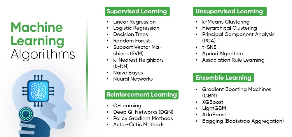
This machine learning cheatsheet serves as a quick reference guide for key concepts and commonly used algorithms in machine learning. It includes essential topics such as supervised learning, unsupervised learning, and reinforcement learning, as well as commonly used algorithms like linear regression and decision trees. This machine learning (ML) cheatsheet is valuable for anyone interested in machine learning.
Table of Contents
Supervised Machine Learning
Supervised Machine Learning Algorithms
Unsupervised Machine Learning
Unsupervised Machine Learning Algorithms
Reinforcement Learning
Reinforcement Learning Algorithms
Supervised Machine Learning
Supervised machine learning is a type of machine learning that trains the algorithms using labeled datasets to predict outcomes.
The main objective of supervised learning is to make algorithms learn an association between input data samples and corresponding outputs after performing multiple training data instances.
Supervised Machine Learning Algorithms
Supervised learning algorithms are categorized into two types of tasks – classification and regression. Below, we have listed commonly used supervised machine learning algorithms, their applications, advantages and disadvantages.
Complex models with multiple layers, capable of learning complex patterns and relationships.
Image classification, natural language processing, speech recognition.
Highly accurate, can handle complex tasks.
Can be computationally expensive, requires careful tuning of hyperparameters.
Unsupervised Machine Learning
Unsupervised machine learning is a type of machine learning that learns patterns and structures within the data without human supervision. Unsupervised learning uses machine learning algorithms to analyze the data and discover underlying patterns within unlabeled data sets.
Unsupervised Machine Learning Algorithms
Unsupervised learning algorithms are categorised into three categories − clustering, association, and dimensionality reduction. Below, we have listed commonly used unsupervised machine learning algorithms, their applications, advantages and disadvantages.
A frequent itemset mining algorithm used to discover associations between items in a dataset.
Market basket analysis, recommendation systems.
Efficient for finding frequent itemsets, can be used for association rule mining.
May not be suitable for large datasets with many items.
t-SNE
Non-linear dimensionality reduction technique that preserves local structure.
Data visualization, clustering, anomaly detection.
Effective for visualizing high-dimensional data in low-dimensional space.
Can be computationally expensive, sensitive to parameters.
UMAP
Another non-linear dimensionality reduction technique that preserves global structure and local relationships.
Data visualization, clustering, anomaly detection.
Often faster and more scalable than t-SNE, preserves global structure well.
May require careful parameter tuning.
Reinforcement Learning
Reinforcement learning is a type of machine learning where an agent (generally a software entity) is trained to interpret the environment by performing actions and monitoring the results. For every good action, the agent gets positive feedback and for every bad action the agent gets negative feedback. It’s inspired by how animals learn from their experiences, making decisions based on the consequences of their actions.
Reinforcement Learning Algorithms
In this section, we have listed some well known reinforcement learning algorithms, their applications, advantages and disadvantages.
Algorithm
Description
Applications
Advantages
Disadvantages
Q-Learning
Off-policy learning algorithm that learns the optimal action-value function.
Game playing, robotics, control systems.
Simple to implement, can handle complex environments.
Can be computationally expensive for large state spaces.
SARSA
On-policy learning algorithm that updates the action-value function based on the current policy.
Game playing, robotics, control systems.
Can handle continuous action spaces, suitable for online learning.
Can be sensitive to exploration-exploitation trade-off.
Deep Q-Networks (DQN)
Combines deep learning with Q-learning, using a neural network to approximate the action-value function.
Atari game playing, robotics, self-driving cars.
Can handle complex environments with large state and action spaces.
Requires careful tuning of hyperparameters, can be computationally expensive.
Policy Gradients
Directly optimizes the policy function to maximize rewards.
Robotics, game playing, natural language processing.
Can handle continuous action spaces, can be more sample efficient than value-based methods.
Can be sensitive to noise and instability.
Actor-Critic
Combines policy-based and value-based methods, using both a policy function and a value function.
Robotics, game playing, natural language processing.
Can be more stable and efficient than pure policy-based or value-based methods.
Requires careful balancing of exploration and exploitation.
Asynchronous Advantage Actor-Critic (A3C)
A parallel version of actor-critic that can handle complex environments with large state spaces.
Robotics, game playing, natural language processing.
Can be more efficient than traditional actor-critic methods, suitable for distributed training.
Todays Artificial Intelligence (AI) has far surpassed the hype of blockchain and quantum computing. This is due to the fact that huge computing resources are easily available to the common man. The developers now take advantage of this in creating new Machine Learning models and to re-train the existing models for better performance and results. The easy availability of High Performance Computing (HPC) has resulted in a sudden increased demand for IT professionals having Machine Learning skills.
In this tutorial, you will learn in detail about −
What is the crux of machine learning?
What are the different types in machine learning?
What are the different algorithms available for developing machine learning models?
What tools are available for developing these models?
What are the programming language choices?
What platforms support development and deployment of Machine Learning applications?
What IDEs (Integrated Development Environment) are available?
How to quickly upgrade your skills in this important area?
Machine Learning – What Todays AI Can Do?
When you tag a face in a Facebook photo, it is AI that is running behind the scenes and identifying faces in a picture. Face tagging is now omnipresent in several applications that display pictures with human faces. Why just human faces? There are several applications that detect objects such as cats, dogs, bottles, cars, etc. We have autonomous cars running on our roads that detect objects in real time to steer the car. When you travel, you use Google Directions to learn the real-time traffic situations and follow the best path suggested by Google at that point of time. This is yet another implementation of object detection technique in real time.
Let us consider the example of Google Translate application that we typically use while visiting foreign countries. Googles online translator app on your mobile helps you communicate with the local people speaking a language that is foreign to you.
There are several applications of AI that we use practically today. In fact, each one of us use AI in many parts of our lives, even without our knowledge. Todays AI can perform extremely complex jobs with a great accuracy and speed. Let us discuss an example of complex task to understand what capabilities are expected in an AI application that you would be developing today for your clients.
Example
We all use Google Directions during our trip anywhere in the city for a daily commute or even for inter-city travels. Google Directions application suggests the fastest path to our destination at that time instance. When we follow this path, we have observed that Google is almost 100% right in its suggestions and we save our valuable time on the trip.
You can imagine the complexity involved in developing this kind of application considering that there are multiple paths to your destination and the application has to judge the traffic situation in every possible path to give you a travel time estimate for each such path. Besides, consider the fact that Google Directions covers the entire globe. Undoubtedly, lots of AI and Machine Learning techniques are in-use under the hoods of such applications.
Considering the continuous demand for the development of such applications, you will now appreciate why there is a sudden demand for IT professionals with AI skills.
In our next chapter, we will learn what it takes to develop AI programs.
Machine Learning – Traditional AI
The journey of AI began in the 1950’s when the computing power was a fraction of what it is today. AI started out with the predictions made by the machine in a fashion a statistician does predictions using his calculator. Thus, the initial entire AI development was based mainly on statistical techniques.
In this chapter, let us discuss in detail what these statistical techniques are.
Statistical Techniques
The development of todays AI applications started with using the age-old traditional statistical techniques. You must have used straight-line interpolation in schools to predict a future value. There are several other such statistical techniques which are successfully applied in developing so-called AI programs. We say so-called because the AI programs that we have today are much more complex and use techniques far beyond the statistical techniques used by the early AI programs.
Some of the examples of statistical techniques that are used for developing AI applications in those days and are still in practice are listed here −
Regression
Classification
Clustering
Probability Theories
Decision Trees
Here we have listed only some primary techniques that are enough to get you started on AI without scaring you of the vastness that AI demands. If you are developing AI applications based on limited data, you would be using these statistical techniques.
However, today the data is abundant. To analyze the kind of huge data that we possess statistical techniques are of not much help as they have some limitations of their own. More advanced methods such as deep learning are hence developed to solve many complex problems.
As we move ahead in this tutorial, we will understand what Machine Learning is and how it is used for developing such complex AI applications.
Machine Learning – What is Machine Learning?
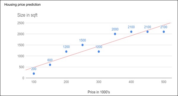
Consider the following figure that shows a plot of house prices versus its size in sq. ft.
After plotting various data points on the XY plot, we draw a best-fit line to do our predictions for any other house given its size. You will feed the known data to the machine and ask it to find the best fit line. Once the best fit line is found by the machine, you will test its suitability by feeding in a known house size, i.e. the Y-value in the above curve. The machine will now return the estimated X-value, i.e. the expected price of the house. The diagram can be extrapolated to find out the price of a house which is 3000 sq. ft. or even larger. This is called regression in statistics. Particularly, this kind of regression is called linear regression as the relationship between X & Y data points is linear.
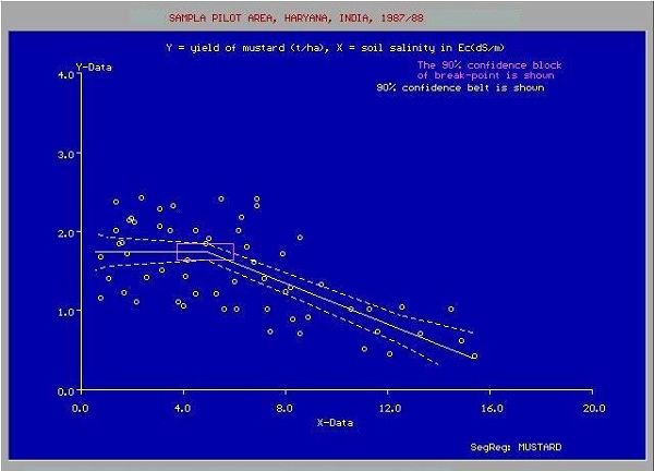
In many cases, the relationship between the X & Y data points may not be a straight line, and it may be a curve with a complex equation. Your task would be now to find out the best fitting curve which can be extrapolated to predict the future values. One such application plot is shown in the figure below.
You will use the statistical optimization techniques to find out the equation for the best fit curve here. And this is what exactly Machine Learning is about. You use known optimization techniques to find the best solution to your problem.
Next, let us look at the different categories of Machine Learning.
Machine Learning – Categories
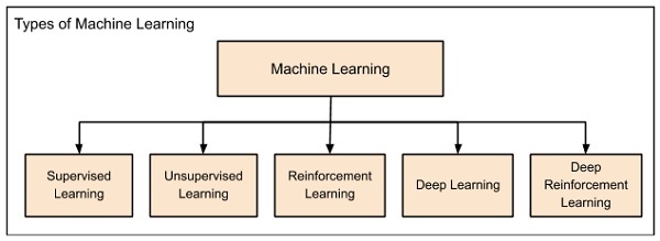
Machine Learning is broadly categorized under the following headings −
Machine learning evolved from left to right as shown in the above diagram.
Initially, researchers started out with Supervised Learning. This is the case of housing price prediction discussed earlier.
This was followed by unsupervised learning, where the machine is made to learn on its own without any supervision.
Scientists discovered further that it may be a good idea to reward the machine when it does the job the expected way and there came the Reinforcement Learning.
Very soon, the data that is available these days has become so humongous that the conventional techniques developed so far failed to analyze the big data and provide us the predictions.
Thus, came the deep learning where the human brain is simulated in the Artificial Neural Networks (ANN) created in our binary computers.
The machine now learns on its own using the high computing power and huge memory resources that are available today.
It is now observed that Deep Learning has solved many of the previously unsolvable problems.
The technique is now further advanced by giving incentives to Deep Learning networks as awards and there finally comes Deep Reinforcement Learning.
Let us now study each of these categories in more detail.
Supervised Learning
Supervised learning is analogous to training a child to walk. You will hold the childs hand, show him how to take his foot forward, walk yourself for a demonstration and so on, until the child learns to walk on his own.
Regression
Similarly, in the case of supervised learning, you give concrete known examples to the computer. You say that for given feature value x1 the output is y1, for x2 it is y2, for x3 it is y3, and so on. Based on this data, you let the computer figure out an empirical relationship between x and y.
Once the machine is trained in this way with a sufficient number of data points, now you would ask the machine to predict Y for a given X. Assuming that you know the real value of Y for this given X, you will be able to deduce whether the machines prediction is correct.
Thus, you will test whether the machine has learned by using the known test data. Once you are satisfied that the machine is able to do the predictions with a desired level of accuracy (say 80 to 90%) you can stop further training the machine.
Now, you can safely use the machine to do the predictions on unknown data points, or ask the machine to predict Y for a given X for which you do not know the real value of Y. This training comes under the regression that we talked about earlier.
Classification
You may also use machine learning techniques for classification problems. In classification problems, you classify objects of similar nature into a single group. For example, in a set of 100 students say, you may like to group them into three groups based on their heights – short, medium and long. Measuring the height of each student, you will place them in a proper group.
Now, when a new student comes in, you will put him in an appropriate group by measuring his height. By following the principles in regression training, you will train the machine to classify a student based on his feature the height. When the machine learns how the groups are formed, it will be able to classify any unknown new student correctly. Once again, you would use the test data to verify that the machine has learned your technique of classification before putting the developed model in production.
Supervised Learning is where the AI really began its journey. This technique was applied successfully in several cases. You have used this model while doing the hand-written recognition on your machine. Several algorithms have been developed for supervised learning. You will learn about them in the following chapters.
Unsupervised Learning
In unsupervised learning, we do not specify a target variable to the machine, rather we ask machine What can you tell me about X?. More specifically, we may ask questions such as given a huge data set X, What are the five best groups we can make out of X? or What features occur together most frequently in X?. To arrive at the answers to such questions, you can understand that the number of data points that the machine would require to deduce a strategy would be very large. In case of supervised learning, the machine can be trained with even about few thousands of data points. However, in case of unsupervised learning, the number of data points that is reasonably accepted for learning starts in a few millions. These days, the data is generally abundantly available. The data ideally requires curating. However, the amount of data that is continuously flowing in a social area network, in most cases data curation is an impossible task.
The following figure shows the boundary between the yellow and red dots as determined by unsupervised machine learning. You can see it clearly that the machine would be able to determine the class of each of the black dots with a fairly good accuracy.
The unsupervised learning has shown a great success in many modern AI applications, such as face detection, object detection, and so on.
Reinforcement Learning
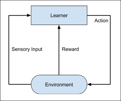
Consider training a pet dog, we train our pet to bring a ball to us. We throw the ball at a certain distance and ask the dog to fetch it back to us. Every time the dog does this right, we reward the dog. Slowly, the dog learns that doing the job rightly gives him a reward and then the dog starts doing the job right way every time in future. Exactly, this concept is applied in Reinforcement type of learning. The technique was initially developed for machines to play games. The machine is given an algorithm to analyze all possible moves at each stage of the game. The machine may select one of the moves at random. If the move is right, the machine is rewarded, otherwise it may be penalized. Slowly, the machine will start differentiating between right and wrong moves and after several iterations would learn to solve the game puzzle with a better accuracy. The accuracy of winning the game would improve as the machine plays more and more games.
The entire process may be depicted in the following diagram −
This technique of machine learning differs from the supervised learning in that you need not supply the labelled input/output pairs. The focus is on finding the balance between exploring the new solutions versus exploiting the learned solutions.
Deep Learning
The deep learning is a model based on Artificial Neural Networks (ANN), more specifically Convolutional Neural Networks (CNN)s. There are several architectures used in deep learning such as deep neural networks, deep belief networks, recurrent neural networks, and convolutional neural networks.
These networks have been successfully applied in solving the problems of computer vision, speech recognition, natural language processing, bioinformatics, drug design, medical image analysis, and games. There are several other fields in which deep learning is proactively applied. The deep learning requires huge processing power and humongous data, which is generally easily available these days.
We will talk about deep learning more in detail in the coming chapters.
Deep Reinforcement Learning
The Deep Reinforcement Learning (DRL) combines the techniques of both deep and reinforcement learning. The reinforcement learning algorithms like Q-learning are now combined with deep learning to create a powerful DRL model. The technique has been with a great success in the fields of robotics, video games, finance and healthcare. Many previously unsolvable problems are now solved by creating DRL models. There is lots of research going on in this area and this is very actively pursued by the industries.
So far, you have got a brief introduction to various machine learning models, now let us explore slightly deeper into various algorithms that are available under these models.
Machine Learning – Supervised
Supervised learning is one of the important models of learning involved in training machines. This chapter talks in detail about the same.
Algorithms for Supervised Learning
There are several algorithms available for supervised learning. Some of the widely used algorithms of supervised learning are as shown below −
k-Nearest Neighbours
Decision Trees
Naive Bayes
Logistic Regression
Support Vector Machines
As we move ahead in this chapter, let us discuss in detail about each of the algorithms.
k-Nearest Neighbours
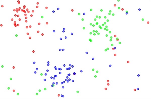
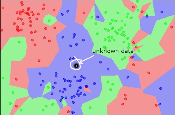
The k-Nearest Neighbours, which is simply called kNN is a statistical technique that can be used for solving for classification and regression problems. Let us discuss the case of classifying an unknown object using kNN. Consider the distribution of objects as shown in the image given below −
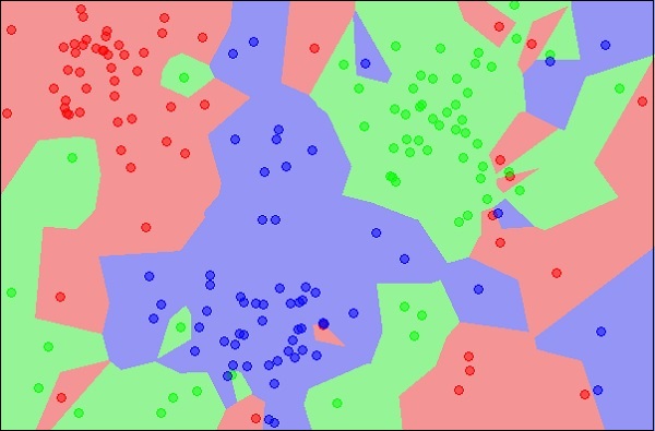
The diagram shows three types of objects, marked in red, blue and green colors. When you run the kNN classifier on the above dataset, the boundaries for each type of object will be marked as shown below −
Now, consider a new unknown object that you want to classify as red, green or blue. This is depicted in the figure below.
As you see it visually, the unknown data point belongs to a class of blue objects. Mathematically, this can be concluded by measuring the distance of this unknown point with every other point in the data set. When you do so, you will know that most of its neighbours are of blue color. The average distance to red and green objects would be definitely more than the average distance to blue objects. Thus, this unknown object can be classified as belonging to blue class.
The kNN algorithm can also be used for regression problems. The kNN algorithm is available as ready-to-use in most of the ML libraries.
Decision Trees
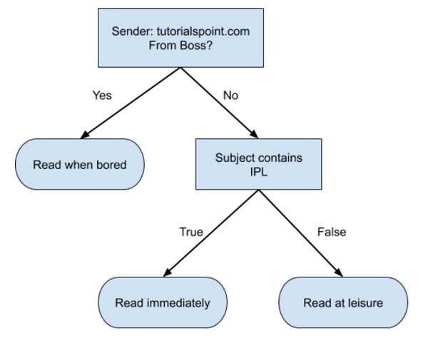
A simple decision tree in a flowchart format is shown below −
You would write a code to classify your input data based on this flowchart. The flowchart is self-explanatory and trivial. In this scenario, you are trying to classify an incoming email to decide when to read it.
In reality, the decision trees can be large and complex. There are several algorithms available to create and traverse these trees. As a Machine Learning enthusiast, you need to understand and master these techniques of creating and traversing decision trees.
Naive Bayes
Naive Bayes is used for creating classifiers. Suppose you want to sort out (classify) fruits of different kinds from a fruit basket. You may use features such as color, size and shape of a fruit, For example, any fruit that is red in color, is round in shape and is about 10 cm in diameter may be considered as Apple. So to train the model, you would use these features and test the probability that a given feature matches the desired constraints. The probabilities of different features are then combined to arrive at a probability that a given fruit is an Apple. Naive Bayes generally requires a small number of training data for classification.
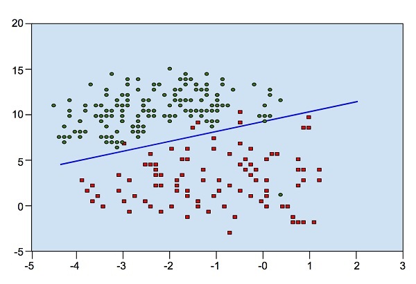
Logistic Regression
Look at the following diagram. It shows the distribution of data points in XY plane.
From the diagram, we can visually inspect the separation of red dots from green dots. You may draw a boundary line to separate out these dots. Now, to classify a new data point, you will just need to determine on which side of the line the point lies.
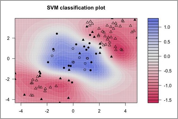
Support Vector Machines
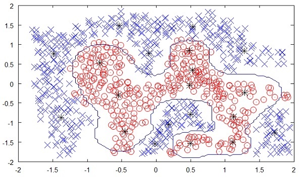
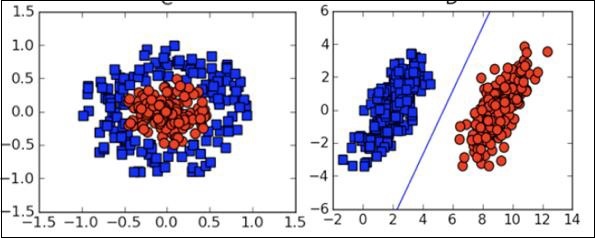
Look at the following distribution of data. Here the three classes of data cannot be linearly separated. The boundary curves are non-linear. In such a case, finding the equation of the curve becomes a complex job.
The Support Vector Machines (SVM) comes handy in determining the separation boundaries in such situations.
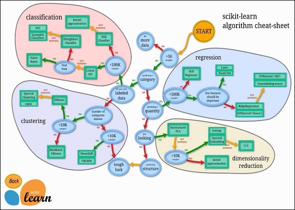
Machine Learning – Scikit-learn Algorithm
Fortunately, most of the time you do not have to code the algorithms mentioned in the previous lesson. There are many standard libraries which provide the ready-to-use implementation of these algorithms. One such toolkit that is popularly used is scikit-learn. The figure below illustrates the kind of algorithms which are available for your use in this library.
The use of these algorithms is trivial and since these are well and field tested, you can safely use them in your AI applications. Most of these libraries are free to use even for commercial purposes.
Machine Learning – Unsupervised
So far what you have seen is making the machine learn to find out the solution to our target. In regression, we train the machine to predict a future value. In classification, we train the machine to classify an unknown object in one of the categories defined by us. In short, we have been training machines so that it can predict Y for our data X. Given a huge data set and not estimating the categories, it would be difficult for us to train the machine using supervised learning. What if the machine can look up and analyze the big data running into several Gigabytes and Terabytes and tell us that this data contains so many distinct categories?
As an example, consider the voters data. By considering some inputs from each voter (these are called features in AI terminology), let the machine predict that there are so many voters who would vote for X political party and so many would vote for Y, and so on. Thus, in general, we are asking the machine given a huge set of data points X, What can you tell me about X?. Or it may be a question like What are the five best groups we can make out of X?. Or it could be even like What three features occur together most frequently in X?.
This is exactly the Unsupervised Learning is all about.
Algorithms for Unsupervised Learning
Let us now discuss one of the widely used algorithms for classification in unsupervised machine learning.
k-means clustering
The 2000 and 2004 Presidential elections in the United States were close very close. The largest percentage of the popular vote that any candidate received was 50.7% and the lowest was 47.9%. If a percentage of the voters were to have switched sides, the outcome of the election would have been different. There are small groups of voters who, when properly appealed to, will switch sides. These groups may not be huge, but with such close races, they may be big enough to change the outcome of the election. How do you find these groups of people? How do you appeal to them with a limited budget? The answer is clustering.
Let us understand how it is done.
First, you collect information on people either with or without their consent: any sort of information that might give some clue about what is important to them and what will influence how they vote.
Then you put this information into some sort of clustering algorithm.
Next, for each cluster (it would be smart to choose the largest one first) you craft a message that will appeal to these voters.
Finally, you deliver the campaign and measure to see if its working.
Clustering is a type of unsupervised learning that automatically forms clusters of similar things. It is like automatic classification. You can cluster almost anything, and the more similar the items are in the cluster, the better the clusters are. In this chapter, we are going to study one type of clustering algorithm called k-means. It is called k-means because it finds k unique clusters, and the center of each cluster is the mean of the values in that cluster.
Cluster Identification
Cluster identification tells an algorithm, Heres some data. Now group similar things together and tell me about those groups. The key difference from classification is that in classification you know what you are looking for. While that is not the case in clustering.
Clustering is sometimes called unsupervised classification because it produces the same result as classification does but without having predefined classes.
Now, we are comfortable with both supervised and unsupervised learning. To understand the rest of the machine learning categories, we must first understand Artificial Neural Networks (ANN), which we will learn in the next chapter.
Machine Learning – Artificial Neural Networks
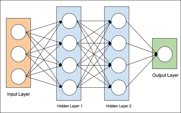
The idea of artificial neural networks was derived from the neural networks in the human brain. The human brain is really complex. Carefully studying the brain, the scientists and engineers came up with an architecture that could fit in our digital world of binary computers. One such typical architecture is shown in the diagram below −
There is an input layer which has many sensors to collect data from the outside world. On the right hand side, we have an output layer that gives us the result predicted by the network. In between these two, several layers are hidden. Each additional layer adds further complexity in training the network, but would provide better results in most of the situations. There are several types of architectures designed which we will discuss now.
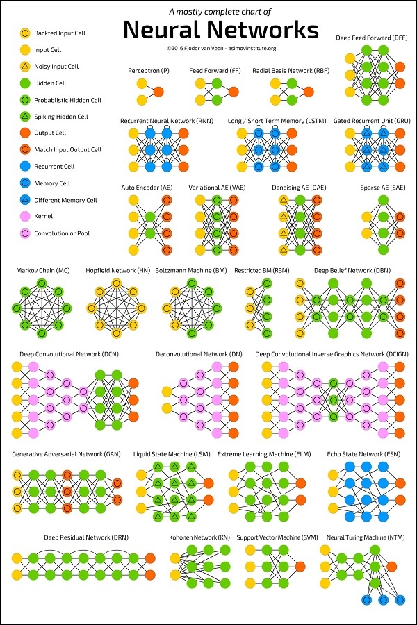
ANN Architectures
The diagram below shows several ANN architectures developed over a period of time and are in practice today.
Each architecture is developed for a specific type of application. Thus, when you use a neural network for your machine learning application, you will have to use either one of the existing architecture or design your own. The type of application that you finally decide upon depends on your application needs. There is no single guideline that tells you to use a specific network architecture.
Machine Learning – Deep Learning
Deep Learning uses ANN. First we will look at a few deep learning applications that will give you an idea of its power.
Applications
Deep Learning has shown a lot of success in several areas of machine learning applications.
Self-driving Cars â The autonomous self-driving cars use deep learning techniques. They generally adapt to the ever changing traffic situations and get better and better at driving over a period of time.
Speech Recognition â Another interesting application of Deep Learning is speech recognition. All of us use several mobile apps today that are capable of recognizing our speech. Apples Siri, Amazons Alexa, Microsofts Cortena and Googles Assistant all these use deep learning techniques.
Mobile Apps â We use several web-based and mobile apps for organizing our photos. Face detection, face ID, face tagging, identifying objects in an image all these use deep learning.
Untapped Opportunities of Deep Learning
After looking at the great success deep learning applications have achieved in many domains, people started exploring other domains where machine learning was not so far applied. There are several domains in which deep learning techniques are successfully applied and there are many other domains which can be exploited. Some of these are discussed here.
Agriculture is one such industry where people can apply deep learning techniques to improve the crop yield.
Consumer finance is another area where machine learning can greatly help in providing early detection on frauds and analyzing customers ability to pay.
Deep learning techniques are also applied to the field of medicine to create new drugs and provide a personalized prescription to a patient.
The possibilities are endless and one has to keep watching as the new ideas and developments pop up frequently.
What is Required for Achieving More Using Deep Learning
To use deep learning, supercomputing power is a mandatory requirement. You need both memory as well as the CPU to develop deep learning models. Fortunately, today we have an easy availability of HPC High Performance Computing. Due to this, the development of the deep learning applications that we mentioned above became a reality today and in the future too we can see the applications in those untapped areas that we discussed earlier.
Now, we will look at some of the limitations of deep learning that we must consider before using it in our machine learning application.
Deep Learning Disadvantages
Some of the important points that you need to consider before using deep learning are listed below −
Black Box approach
Duration of Development
Amount of Data
Computationally Expensive
We will now study each one of these limitations in detail.
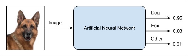
Black Box approach
An ANN is like a blackbox. You give it a certain input and it will provide you a specific output. The following diagram shows you one such application where you feed an animal image to a neural network and it tells you that the image is of a dog.
Why this is called a black-box approach is that you do not know why the network came up with a certain result. You do not know how the network concluded that it is a dog? Now consider a banking application where the bank wants to decide the creditworthiness of a client. The network will definitely provide you an answer to this question. However, will you be able to justify it to a client? Banks need to explain it to their customers why the loan is not sanctioned?
Duration of Development
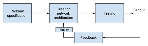
The process of training a neural network is depicted in the diagram below −
You first define the problem that you want to solve, create a specification for it, decide on the input features, design a network, deploy it and test the output. If the output is not as expected, take this as a feedback to restructure your network. This is an iterative process and may require several iterations until the time network is fully trained to produce desired outputs.
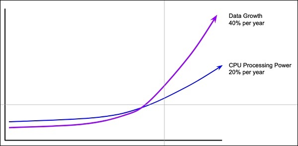
Amount of Data
The deep learning networks usually require a huge amount of data for training, while the traditional machine learning algorithms can be used with a great success even with just a few thousands of data points. Fortunately, the data abundance is growing at 40% per year and CPU processing power is growing at 20% per year as seen in the diagram given below −
Computationally Expensive
Training a neural network requires several times more computational power than the one required in running traditional algorithms. Successful training of deep Neural Networks may require several weeks of training time.
In contrast to this, traditional machine learning algorithms take only a few minutes/hours to train. Also, the amount of computational power needed for training deep neural network heavily depends on the size of your data and how deep and complex the network is?
After having an overview of what Machine Learning is, its capabilities, limitations, and applications, let us now dive into learning Machine Learning.
Machine Learning – Skills
Machine Learning has a very large width and requires skills across several domains. The skills that you need to acquire for becoming an expert in Machine Learning are listed below −
Statistics
Probability Theories
Calculus
Optimization techniques
Visualization
Necessity of Various Skills of Machine Learning
To give you a brief idea of what skills you need to acquire, let us discuss some examples −
Mathematical Notation
Most of the machine learning algorithms are heavily based on mathematics. The level of mathematics that you need to know is probably just a beginner level. What is important is that you should be able to read the notation that mathematicians use in their equations. For example – if you are able to read the notation and comprehend what it means, you are ready for learning machine learning. If not, you may need to brush up your mathematics knowledge.
If you can read and understand the above, you are all set.
Visualization
In many cases, you will need to understand the various types of visualization plots to understand your data distribution and interpret the results of the algorithms output.
Besides the above theoretical aspects of machine learning, you need good programming skills to code those algorithms.
So what does it take to implement ML? Let us look into this in the next chapter.
Machine Learning – Implementing
To develop ML applications, you will have to decide on the platform, the IDE and the language for development. There are several choices available. Most of these would meet your requirements easily as all of them provide the implementation of AI algorithms discussed so far.
If you are developing the ML algorithm on your own, the following aspects need to be understood carefully −
The language of your choice â this essentially is your proficiency in one of the languages supported in ML development.
The IDE that you use â This would depend on your familiarity with the existing IDEs and your comfort level.
Development platform â There are several platforms available for development and deployment. Most of these are free-to-use. In some cases, you may have to incur a license fee beyond a certain amount of usage. Here is a brief list of choice of languages, IDEs and platforms for your ready reference.
Language Choice
Here is a list of languages that support ML development −
Python
R
Matlab
Octave
Julia
C++
C
This list is not essentially comprehensive; however, it covers many popular languages used in machine learning development. Depending upon your comfort level, select a language for the development, develop your models and test.
IDEs
Here is a list of IDEs which support ML development −
R Studio
Pycharm
iPython/Jupyter Notebook
Julia
Spyder
Anaconda
Rodeo
Google Colab
The above list is not essentially comprehensive. Each one has its own merits and demerits. The reader is encouraged to try out these different IDEs before narrowing down to a single one.
Platforms
Here is a list of platforms on which ML applications can be deployed −
IBM
Microsoft Azure
Google Cloud
Amazon
Mlflow
Once again this list is not exhaustive. The reader is encouraged to sign-up for the abovementioned services and try them out themselves.
Machine Learning – Conclusion
This tutorial has introduced you to Machine Learning. Now, you know that Machine Learning is a technique of training machines to perform the activities a human brain can do, albeit bit faster and better than an average human-being. Today we have seen that the machines can beat human champions in games such as Chess, AlphaGO, which are considered very complex. You have seen that machines can be trained to perform human activities in several areas and can aid humans in living better lives.
Machine Learning can be a Supervised or Unsupervised. If you have lesser amount of data and clearly labelled data for training, opt for Supervised Learning. Unsupervised Learning would generally give better performance and results for large data sets. If you have a huge data set easily available, go for deep learning techniques. You also have learned Reinforcement Learning and Deep Reinforcement Learning. You now know what Neural Networks are, their applications and limitations.
Finally, when it comes to the development of machine learning models of your own, you looked at the choices of various development languages, IDEs and Platforms. Next thing that you need to do is start learning and practicing each machine learning technique. The subject is vast, it means that there is width, but if you consider the depth, each topic can be learned in a few hours. Each topic is independent of each other. You need to take into consideration one topic at a time, learn it, practice it and implement the algorithm/s in it using a language choice of yours. This is the best way to start studying Machine Learning. Practicing one topic at a time, very soon you would acquire the width that is eventually required of a Machine Learning expert.
Data in machine learning are broadly categorized into two types − numerical (quantitative) and categorical (qualitative) data. The numerical data can be measured, counted or given a numerical value, for example, age, height, income, etc. The categorical data is non-numeric data that can be arranged in categories with or without meaningful order, for example, gender, blood group, etc.
Further, the numerical data can be categorized into discrete and continuous data. The categorical data can also be categorized into two types − nominal and ordinal. Let’s understand these types of data in machine learning in detail.
What is Data in Machine Learning?
Data in machine learning is a set of observations or measurement that are used to train, validate and test a machine learning model. Data is very crucial in machine learning because it is the foundation of creating accurate machine learning model.
What are Types of Data?
The data used in machine learning can be broadly categorized into two types −
The numerical (quantitative) data is data that can be measured, counted or given a numerical value. The examples of numerical data are age, height, income, number of students in class, number of books in a shelf, shoe size, etc.
The numerical data can be categorized into the folloiwng two types −
Discrete Data
Continuous Data
1. Discrete Data
The discrete data is numerical data that is countable, finite, and can only take certain values, usually whole numbers. Examples of discrete data are number of students in class, number of books in a shelf, shoe size, number of ducks in a pond, etc.
2. Continuous Data
The continuous data is numerical data that can take any value within a specified range including fractions and decimals. Examples of continuous data are age, height, weight, income, time, temperature, etc.
What is true zero?
True zero represents the absence of the quantity being measured. For example, height, weight, age, temperature in Kelvin are examples of data with true zero. As the height with 0 CM represents the absolute absence of height, 0K temperature represents no heat. But temperature in Celsius (or Fahrenheit) is an example of data with false zero.
We can categorize the numerical data into the following two types on basis of true zero −
interval data − quantitative data with equal intervals between data points. Examples are temperature (Fahrenheit), temperature (Celsius), pH, SAT score (200-800), credit score (300-850), etc.
ratio data − same as interval data but with true zero. Examples are weight in KG, number of students, income, speed, etc.
Categorical (Qualitative) Data
The categorical (qualitative) data can be categorized with or without a meaningful order. For example, gender, blood group, hair color, nationality, the school grades, level of education, range of income, ratings, etc.
The categorical data can be divided into the folloiwng two types −
Nominal Data
Ordinal Data
1. Nominal Data
The nominal data is categorical data that can not be arranged in an order or rank. The examples of nominal data are gender, blood group, hair color, nationality, etc.
2. Ordinal Data
The ordinal data is categorical data can be ordered or ranked with a specific attribute. The examples of ordinal data are the school grades, level of education, range of income, ratings, etc.
The Four Levels of Data Measurement
We can categorized data into four level − nominal, ordinal, interval, and ratio. These levels of measurement are divided on basis of the following four features −
Categories − data can be categorized but not in an order.
Rank Order − data can be categorized with some meaningful order.
Equal Difference − The difference between subsequent data remains same.
True Zero − it represents the absence of quantity being measured.
The following table highlights how the four level of measurement are associated with the above discussed four features.
Nominal
Ordinal
Interval
Ratio
Categories
Yes
Yes
Yes
Yes
Rank Order
Yes
Yes
Yes
Equal Difference
Yes
Yes
True Zero
Yes
The nominal data is categorical data with no meaningful order whereas ordinal data is a categorical data with meaningful order. The concept of true zero plays role to differentiate interval and ratio data. Ratio data is same as interval data but it includes true zero.
Monetizing machine learning refers to transforming machine learning projects into profitable web applications. Monetizing an ML project involves many steps including problem understanding, ML model development, web application development, model integration to web application, serverless cloud deployment of the final web app and finally monetizing the application.
The idea behind monetizing machine learning project is simple. What we will do? We will build a simple fast SaaS application for project and monetize it.
Creating a Software as a Service (SaaS) is a good choice for its many benefits such as reduced costs, scalability, ease of management, etc.
To monetize, we can consider subscription based pricing, premium features, API access, advertising, custom service, etc.
Let’s understand how to transform a machine learning project into a web application and monetize it.
Understanding the Problems
Take a real-world problem and do research on whether we can solve the problem using machine learning. If yes, find out if it is feasible to implement the solution using all your resources.
Who will benefit from the ML solution − the final end users? Who is the end user of the final machine learning application? Understanding the users is very important when you are analyzing a real-world problem.
The problem falls under what type of task in the machine learning context. What types of models can be used to solve the problem? Whether the problem can be solved using regression, classification, or clustering models. A proper understanding of the problem will help you to find the answers of these questions.
What would be the business model? Whether web application of mobile application, API sale or combination of two or more?
What type of data we have? Structured or unstructured. Analyze the data properly before going to solve the problem. It will help to decide what type of machine learning approach you should follow.
What computational resources you have? How to develop ML models? − on premise or cloud-based.
Understand the real world problem properly that you want to solve.
Defining the Solution
What will be the final solution of the problem?
Define the solution − how you will present the solution to the end user whether you will develop a web application, mobile app, API or a combination.
What is the business model?
Define your business model. What type of product for machine leaning model you want to create? One of the best solution is to create a software as a service (SaaS). You can consider for PaaS, AIaaS, Mobile Applications, API Service, and Selling ML APIs, etc.
Building a web application using serverless technology is a good choice to showcase your machine leaning application or solution. It is also easy to monetize your solution later on.
When you decide how you bring the solution to world, the next step is defining the core features of your machine learning solution. User interaction with the application, navigation, login, security, data privacy, etc., should be defined before diving into building the machine learning model.
Developing Machine Learning Model
The next step is to start developing your machine learning model. But before actually starting, you need to understand the machine learning models in detail. Without having a good knowledge of ML models you can’t be able to decide which model to select for your problem.
Understand Machine Learning Models
It is very important to understand different types of machine learning models and how to choose the right one for your project. Understanding the ML models will help select an appropriate model for your machine learning application.
Understanding that the underlined solution will fall under a particular machine learning task will help you decide on the proper model. Suppose your solution falls under the classification, then you have many choices of machine learning model. You can apply Naïve base, logistic regression, k-nearest neighbor, decision trees, and many more. So having a proper understanding of models is required before going to make your hands dirty with data and model training.
Types of ML Models
You should have a good understanding of the following types of machine learning models −
The most important step in building a machine learning model is to select the right one that solves your business problem. While selecting the right ML model, you should consider different factors such as −
Data characteristics − consider the nature of data (structured, unstructured, time series data) to select a suitable model.
Problem type − determine whether your problem is regression, classification or other task.
Model complexity − determine the optimal model complexity to avoid the overfitting or under fitting.
Computational resources − consider the computational resources to choose a complex or simple model.
Desired outcome − consider it to perform the model evaluation.
Train Machine Learning Model
After selecting the right model for your machine learning problem, the next is to start building the actual machine learning model. There are different ways to build an ML model. The easiest way is to use a pre-trained model and custom train on your own datasets.
Pre-trained models − Pre-trained models are machine learning models that are trained with huge datasets. If your data is similar to the datasets on which the pre-trained models are trained, you can select them for your solution. In such cases, you need only to build a web or mobile application and deploy it on the cloud for worldwide users.
Fine-Tuning Pre-Trained Model − You can consider fine-tuning a pre-trained model on your custom datasets. You can fine-tune any publicly available model using machine learning libraries/ frameworks such as TensorFlow/ Keras, PyTorch, etc. You can also consider some online platforms such as AWS Sagemaker, Vertex AI, IBM Watson Studio, Azure Machine Learning, etc. for fine-tuning purposes.
Build from Scratch − You can consider building a machine learning model from scratch if you have all the required resources. It may take more time compared to the above two ways but may cost a little less.
Amazon SageMaker is a cloud-based machine-learning platform to create, train, evaluate, and deploy etc. machine-learning models on the cloud.
Evaluate Model
You have trained your ML model on your custom dataset. Now you have to evaluate the model on some new data to check whether the model is performing as per our desired outcomes or not.
For evaluating your machine learning model, you can calculate the metrics such as accuracy, precision, recall, f1 score, confusion matrix, etc. Based on these metrics, you can decide on a further course of action − finalizing the current model or going back with training again.
You can consider ensemble methods, combining multiple models (bagging and boosting) to improve model performance and reduce overfitting.
Deploy Demo Model online
Before building a full-fledged web application and deploying it on a cloud server, it is advised to deploy your machine learning model online. There are many free hosting providers where you can deploy your machine learning model and get feedback from the real time users. You can consider the following providers for this purpose −
Hugging Face Space
Streamlit Cloud
Heroku
Creating Machine Learning Web Applications
As of now, you have developed your ML model and deployed the demo model online. Your model is working perfectly. Now you are ready to build a full-fledged machine learning web or mobile application.
You can consider the following technology stack to build web applications −
Python frameworks – Flask, Django, FastAPI, etc.
Web development (frontend) concepts − HTML, CSS, JavaScript
Integrating machine learning models − how to integrate using APIs or libraries − Rest API
Deploying on the Serverless Cloud
Deploying your ML application on a serverless cloud will open doors to monetize your application. It will reach a worldwide audience. Choosing a cloud platform is a good idea to host your app. Going serverless can benefit you with reduced costs, scalability, ease of management, etc.
The following is a list of some well-known serverless cloud service providers best for your machine learning web applications −
You can use services like EC2 for computing power and S3 for storage.
Monetizing Your Machine Learning Applications
Now, your machine learning application is live on the cloud. You can promote, and market to your users. You can give them special offers to use your application.
Your machine learning application can reach to any corner of the world. When you get enough user, you can think about monetizing your application. There are different strategies to monetize ML web application including subscription model, pay-per-use pricing, advertising, premium features, etc.
Subscription Model − Subscription-based pricing tiers (e.g., basic, premium, enterprise).
Freemium Model − Offer a free version with limited features, and charge for advanced features.
API Access − Charge businesses to access your AI tools via an API.
Advertising − you can also consider putting advertisement on your application but keep it in mind that advertisements will distort your application’s premium look.
Marketing and Sales
Marketing and sales are important to grow any business. Continuous marketing is required for a better sale of the product.
You can sell your Machine Learning application APIs on different online API marketplaces.
You can consider the following API Marketplaces −
RapidAPI
APILayer
AWS Marketplace
Infosys API Marketplace
IBM API Connect
Monetizing machine learning has now become easy but more competitive. Monetizing the ML application needs a detailed market analysis before starting the building application. Each step of the machine learning software development needs deep research. Building a minimum viable product (MVP) and testing it before building a full-fledged web application is advisable.
Data leakage is a common problem in machine learning that occurs when information from outside the training dataset is used to create or evaluate a model. This can lead to overfitting, where the model is too closely tailored to the training data and performs poorly on new data.
There are two main types of data leakage: Target Leakage and Train-test Contamination
Target Leakage
Target leakage occurs when features that are not available during prediction are used to create the model. For example, if we are predicting whether a customer will churn, and we include the customer’s cancellation date as a feature, then the model will have access to information that would not be available in practice. This can lead to unrealistically high accuracy during training and poor performance on new data.
Train-test Contamination
Train-test contamination occurs when information from the test set is inadvertently used in the training process. For example, if we normalize the data based on the mean and standard deviation of the entire dataset instead of just the training set, then the model will have access to information that would not be available in practice. This can lead to overly optimistic estimates of model performance.
How to Prevent Data Leakage?
To prevent data leakage, it is important to carefully preprocess the data and ensure that no information from the test set is used in the training process. Some strategies for preventing data leakage include −
Splitting the data into separate training and test sets before doing any preprocessing or feature engineering.
Only using features that would be available at the time of prediction.
Using cross-validation to evaluate model performance instead of a single train-test split.
Ensuring that all preprocessing steps (such as normalization or scaling) are applied to the training set only and then using the same transformations on the test set.
Being aware of any potential sources of leakage, such as date or time-based features, and handling them appropriately.
Implementation in Python
Here is an example in which we will be using Sklearn breast cancer dataset and ensure that no information from the test set is leaked into the model during training −
Example
from sklearn.datasets import load_breast_cancer
from sklearn.model_selection import train_test_split
from sklearn.pipeline import Pipeline
from sklearn.preprocessing import StandardScaler
from sklearn.svm import SVC

# Load the breast cancer dataset
data = load_breast_cancer()# Separate features and labels
X, y = data.data, data.target

# Split the data into train and test sets
X_train, X_test, y_train, y_test = train_test_split(X, y, test_size=0.2, random_state=42)# Define the pipeline
pipeline = Pipeline([('scaler', StandardScaler()),('svm', SVC())])# Fit the pipeline on the train set
pipeline.fit(X_train, y_train)# Make predictions on the test set
y_pred = pipeline.predict(X_test)# Evaluate the model performance
accuracy = accuracy_score(y_test, y_pred)print("Accuracy:", accuracy)
Output
When you execute this code, it will produce the following output −
MLOps (Machine Learning Operations) is a set of practices and tools that combine software engineering, data science, and operations to enable the automated deployment, monitoring, and management of machine learning models in production environments.
MLOps addresses the challenges of managing and scaling machine learning models in production, which include version control, reproducibility, model deployment, monitoring, and maintenance. It aims to streamline the entire machine learning lifecycle, from data preparation and model training to deployment and maintenance.
MLOps Best Practices
MLOps involves a number of key practices and tools, including −
Version control − This involves tracking changes to code, data, and models using tools like Git to ensure reproducibility and maintain a history of all changes.
Continuous integration and delivery (CI/CD) − This involves automating the process of building, testing, and deploying machine learning models using tools like Jenkins, Travis CI, or CircleCI.
Containerization − This involves packaging machine learning models and dependencies into containers using tools like Docker or Kubernetes, which enables easy deployment and scaling of models in production environments.
Model serving − This involves setting up a server to host machine learning models and serving predictions on incoming data.
Monitoring and logging − This involves tracking the performance of machine learning models in production environments using tools like Prometheus or Grafana, and logging errors and alerts to enable proactive maintenance.
Automated testing − This involves automating the testing of machine learning models to ensure they are accurate and robust.
Python Libraries for MLOps
Python has a number of libraries and tools that can be used for MLOps, including −
Scikit-learn − A popular machine learning library that provides tools for data preprocessing, model selection, and evaluation.
TensorFlow − A widely used open-source platform for building and deploying machine learning models.
Keras − A high-level neural networks API that can run on top of TensorFlow.
PyTorch − A deep learning framework that provides tools for building and deploying neural networks.
MLflow − An open-source platform for managing the machine learning lifecycle that provides tools for tracking experiments, packaging code and models, and deploying models in production.
Kubeflow − A machine learning toolkit for Kubernetes that provides tools for managing and scaling machine learning workflows.
Entropy is a concept that originates from thermodynamics and was later applied in various fields, including information theory, statistics, and machine learning. In machine learning, entropy is used as a measure of the impurity or randomness of a set of data. Specifically, entropy is used in decision tree algorithms to decide how to split the data to create a more homogeneous subset. In this article, we will discuss entropy in machine learning, its properties, and its implementation in Python.
Entropy is defined as a measure of disorder or randomness in a system. In the context of decision trees, entropy is used as a measure of the impurity of a node. A node is considered pure if all the examples in it belong to the same class. In contrast, a node is impure if it contains examples from multiple classes.
To calculate entropy, we need to first define the probability of each class in the data set. Let p(i) be the probability of an example belonging to class i. If we have k classes, then the total entropy of the system, denoted by H(S), is calculated as follows −
H(S)=−sum(p(i)∗log2(p(i)))
where the sum is taken over all k classes. This equation is called the Shannon entropy.
For example, suppose we have a dataset with 100 examples, of which 60 belong to class A and 40 belong to class B. Then the probability of class A is 0.6 and the probability of class B is 0.4. The entropy of the dataset is then −
H(S)=−(0.6×log2(0.6)+0.4×log2(0.4))=0.971
If all the examples in the dataset belong to the same class, then the entropy is 0, indicating a pure node. On the other hand, if the examples are evenly distributed across all classes, then the entropy is high, indicating an impure node.
In decision tree algorithms, entropy is used to determine the best split at each node. The goal is to create a split that results in the most homogeneous subsets. This is done by calculating the entropy of each possible split and selecting the split that results in the lowest total entropy.
For example, suppose we have a dataset with two features, X1 and X2, and the goal is to predict the class label, Y. We start by calculating the entropy of the entire dataset, H(S). Next, we calculate the entropy of each possible split based on each feature. For example, we could split the data based on the value of X1 or the value of X2. The entropy of each split is calculated as follows −
H(X1)=p1×H(S1)+p2×H(S2)H(X2)=p3×H(S3)+p4×H(S4)
where p1, p2, p3, and p4 are the probabilities of each subset; and H(S1), H(S2), H(S3), and H(S4) are the entropies of each subset.
We then select the split that results in the lowest total entropy, which is given by −
Hsplit=H(X1)ifH(X1)≤H(X2);elseH(X2)
This split is then used to create the child nodes of the decision tree, and the process is repeated recursively until all nodes are pure or a stopping criterion is met.
Example
Let’s take an example to understand how it can be implemented in Python. Here we will use the “iris” dataset −
from sklearn.datasets import load_iris
import numpy as np

# Load iris dataset
iris = load_iris()# Extract features and target
X = iris.data
y = iris.target

# Define a function to calculate entropydefentropy(y):
   n =len(y)
   _, counts = np.unique(y, return_counts=True)
   probs = counts / n
   return-np.sum(probs * np.log2(probs))# Calculate the entropy of the target variable
target_entropy = entropy(y)print(f"Target entropy: {target_entropy:.3f}")
The above code loads the iris dataset, extracts the features and target, and defines a function to calculate entropy. The entropy() function takes a vector of target values and returns the entropy of the set.
The function first calculates the number of examples in the set and the count of each class. It then calculates the proportion of each class and uses these to calculate the entropy of the set using the entropy formula. Finally, the code calculates the entropy of the target variable in the iris dataset and prints it to the console.
Output
When you execute this code, it will produce the following output −
In machine learning, we use P-value to test the null hypothesis that there is no significant relationship between two variables. For example, if we have a dataset of house prices and we want to determine whether there is a significant relationship between the size of the house and its price, we can use P-value to test this hypothesis.
To understand the concept of P-value in machine learning, we need to first understand the concept of null hypothesis and alternative hypothesis. The null hypothesis is the hypothesis that there is no significant relationship between the two variables, while the alternative hypothesis is the opposite of the null hypothesis, which states that there is a significant relationship between the two variables.
Once we have defined our null hypothesis and alternative hypothesis, we can use P-value to test the significance of our hypothesis. The P-value is the probability of obtaining the observed result or a more extreme result, assuming that the null hypothesis is true.
If the P-value is less than the significance level (usually set at 0.05), then we reject the null hypothesis and accept the alternative hypothesis. This means that there is a significant relationship between the two variables. On the other hand, if the P-value is greater than the significance level, then we fail to reject the null hypothesis and conclude that there is no significant relationship between the two variables.
Implementation of P-value in Python
Python provides several libraries for statistical analysis and hypothesis testing. One of the most popular libraries for statistical analysis is the scipy library. The scipy library provides a function called ttest_ind() that can be used to calculate the P-value for two independent samples.
To demonstrate the implementation of p-value in Machine Learning, we will use the breast cancer dataset provided by scikit-learn. The goal of this dataset is to predict whether a breast tumor is malignant or benign based on various features such as the tumor’s radius, texture, perimeter, area, smoothness, compactness, concavity, and symmetry.
First, we will load the dataset and split it into training and testing sets −
from sklearn.datasets import load_breast_cancer
from sklearn.model_selection import train_test_split

data = load_breast_cancer()
X = data.data
y = data.target

X_train, X_test, y_train, y_test = train_test_split(X, y, test_size=0.2, random_state=42)
Next, we will use the SelectKBest class from scikit-learn to select the top k features based on their p-values. Here, we will select the top 5 features −
from sklearn.feature_selection import SelectKBest, f_classif
k =5
selector = SelectKBest(score_func=f_classif, k=k)
X_train_new = selector.fit_transform(X_train, y_train)
X_test_new = selector.transform(X_test)
The SelectKBest class takes a score function as input to calculate the p-values for each feature. We use the f_classif function, which is the ANOVA F-value between each feature and the target variable. The k parameter specifies the number of top features to select.
After fitting the selector on the training data, we transform the data to keep only the top k features using the fit_transform() method. We also transform the testing data to keep only the selected features using the transform() method.
We can now train a model on the selected features and evaluate its performance −
from sklearn.linear_model import LogisticRegression
from sklearn.metrics import accuracy_score

model = LogisticRegression()
model.fit(X_train_new, y_train)
y_pred = model.predict(X_test_new)

accuracy = accuracy_score(y_test, y_pred)print(f"Accuracy: {accuracy:.2f}")
In this example, we trained a logistic regression model on the top 5 selected features and evaluated its performance using accuracy. However, the p-value can also be used for hypothesis testing to determine whether a feature is statistically significant or not.
For example, to test the hypothesis that the mean radius feature is significant, we can use the ttest_ind() function from the scipy.stats module −
Overfitting occurs when a model learns the noise in the training data, rather than the underlying patterns. This causes the model to perform well on the training data, but poorly on new data. Essentially, the model becomes too specialized to the training data, and is unable to generalize to new data.
Overfitting is a common problem when using complex models, such as deep neural networks. These models have many parameters, and are able to fit the training data very closely. However, this often comes at the expense of generalization performance.
Causes of Overfitting
There are several factors that can contribute to overfitting −
Complex models − As mentioned earlier, complex models are more likely to overfit than simpler models. This is because they have more parameters, and are able to fit the training data more closely.
Limited training data − When there is not enough training data, it becomes difficult for the model to learn the underlying patterns, and it may instead learn the noise in the data.
Unrepresentative training data − If the training data is not representative of the problem that the model is trying to solve, the model may learn irrelevant patterns that do not generalize well to new data.
Lack of regularization − Regularization is a technique used to prevent overfitting by adding a penalty term to the cost function. If this penalty term is not present, the model is more likely to overfit.
Techniques to Prevent Overfitting
There are several techniques that can be used to prevent overfitting in machine learning −
Cross-validation − Cross-validation is a technique used to evaluate a model’s performance on new, unseen data. It involves dividing the data into several subsets, and using each subset in turn as a validation set, while training on the remaining data. This helps to ensure that the model generalizes well to new data.
Early stopping − Early stopping is a technique used to prevent a model from overfitting by stopping the training process before it has converged completely. This is done by monitoring the validation error during training, and stopping when the error stops improving.
Regularization − Regularization is a technique used to prevent overfitting by adding a penalty term to the cost function. The penalty term encourages the model to have smaller weights, and helps to prevent it from fitting the noise in the training data.
Dropout − Dropout is a technique used in deep neural networks to prevent overfitting. It involves randomly dropping out some of the neurons during training, which forces the remaining neurons to learn more robust features.
Example
Here is an implementation of early stopping and L2 regularization in Python using Keras −
from keras.models import Sequential
from keras.layers import Dense
from keras.callbacks import EarlyStopping
from keras import regularizers

# define the model architecture
model = Sequential()
model.add(Dense(64, input_dim=X_train.shape[1], activation='relu', kernel_regularizer=regularizers.l2(0.01)))
model.add(Dense(32, activation='relu', kernel_regularizer=regularizers.l2(0.01)))
model.add(Dense(1, activation='sigmoid'))# compile the model
model.compile(loss='binary_crossentropy', optimizer='adam', metrics=['accuracy'])# set up early stopping callback
early_stopping = EarlyStopping(monitor='val_loss', patience=5)# train the model with early stopping and L2 regularization
history = model.fit(X_train, y_train, validation_split=0.2, epochs=100, batch_size=64, callbacks=[early_stopping])
In this code, we have used the Sequential model in Keras to define the model architecture, and we have added L2 regularization to the first two layers using the kernel_regularizer argument. We have also set up an early stopping callback using the EarlyStopping class in Keras, which will monitor the validation loss and stop training if it stops improving for 5 epochs.
During training, we pass in the X_train and y_train data as well as a validation split of 0.2 to monitor the validation loss. We also set a batch size of 64 and train for a maximum of 100 epochs.
Output
When you execute this code, it will produce an output like the one shown below −
In machine learning, regularization is a technique used to prevent overfitting, which occurs when a model is too complex and fits the training data too well, but fails to generalize to new, unseen data. Regularization introduces a penalty term to the cost function, which encourages the model to have smaller weights and a simpler structure, thereby reducing overfitting.
There are several types of regularization techniques commonly used in machine learning, including L1 and L2 regularization, dropout regularization, and early stopping. In this article, we will focus on L1 and L2 regularization, which are the most commonly used techniques.
L1 Regularization
L1 regularization, also known as Lasso regularization, is a technique that adds a penalty term to the cost function, equal to the absolute value of the sum of the weights. The formula for the L1 regularization penalty is −
λ×Σ|wi|
where is a hyperparameter that controls the strength of the regularization, and is the i-th weight in the model.
The effect of the L1 regularization penalty is to encourage the model to have sparse weights, that is, to eliminate the weights that have little or no impact on the output. This has the effect of simplifying the model and reducing overfitting.
Example
To implement L1 regularization in Python, we can use the Lasso class from the scikit-learn library. Here is an example of how to use L1 regularization for linear regression −
from sklearn.linear_model import Lasso
from sklearn.datasets import load_boston
from sklearn.model_selection import train_test_split
from sklearn.metrics import mean_squared_error

# Load the Boston Housing dataset
boston = load_boston()# Split the data into training and test sets
X_train, X_test, y_train, y_test = train_test_split(boston.data, boston.target, test_size=0.2, random_state=42)# Create a Lasso model with L1 regularization
lasso = Lasso(alpha=0.1)# Train the model on the training data
lasso.fit(X_train, y_train)# Make predictions on the test data
y_pred = lasso.predict(X_test)# Calculate the mean squared error of the predictions
mse = mean_squared_error(y_test, y_pred)print("Mean squared error:", mse)
In this example, we load the Boston Housing dataset, split it into training and test sets, and create a Lasso model with L1 regularization using an alpha value of 0.1. We then train the model on the training data and make predictions on the test data. Finally, we calculate the mean squared error of the predictions.
Output
When you execute this code, it will produce the following output −
Mean squared error: 25.155593753934173
L2 Regularization
L2 regularization, also known as Ridge regularization, is a technique that adds a penalty term to the cost function, equal to the square of the sum of the weights. The formula for the L2 regularization penalty is −
λ×Σ(wi)2
where is a hyperparameter that controls the strength of the regularization, and wi is the ith weight in the model.
The effect of the L2 regularization penalty is to encourage the model to have small weights, that is, to reduce the magnitude of all the weights in the model. This has the effect of smoothing the model and reducing overfitting.
Example
To implement L2 regularization in Python, we can use the Ridge class from the scikit-learn library. Here is an example of how to use L2 regularization for linear regression −
from sklearn.linear_model import Ridge
from sklearn.model_selection import train_test_split
from sklearn.metrics import mean_squared_error
from sklearn.datasets import load_boston
from sklearn.preprocessing import StandardScaler
import numpy as np

# load the Boston housing dataset
boston = load_boston()# create feature and target arrays
X = boston.data
y = boston.target

# standardize the feature data
scaler = StandardScaler()
X = scaler.fit_transform(X)# split the data into training and testing sets
X_train, X_test, y_train, y_test = train_test_split(X, y, test_size=0.2, random_state=42)# define the Ridge regression model with L2 regularization
model = Ridge(alpha=0.1)# fit the model on the training data
model.fit(X_train, y_train)# make predictions on the testing data
y_pred = model.predict(X_test)# calculate the mean squared error
mse = mean_squared_error(y_test, y_pred)print("Mean Squared Error: ", mse)
In this example, we first load the Boston housing dataset and split it into training and testing sets. We then standardize the feature data using a StandardScaler.
Next, we define the Ridge regression model and set the alpha parameter to 0.1, which controls the strength of the L2 regularization.
We fit the model on the training data and make predictions on the testing data. Finally, we calculate the mean squared error to evaluate the performance of the model.
Output
When you execute this code, it will produce the following output −