What is K-Ary Tree?
K-ary tree also known as K-way or N-ary tree is a tree data structure in which each node has at most K children. The value of K is fixed for a given tree. The value of K can be 2, 3, 4, 5, etc.
For example, a binary tree is a 2-ary tree, a ternary tree is a 3-ary tree, and so on.
Characteristics of K-Ary Tree
Following are the characteristics of K-ary tree:
- K : This number represents the maximum number of children a node can have.
- Height : The height of a K-ary tree is the maximum number of edges on the longest path between the root node and a leaf node.
- Level: The level of a node is the number of edges on the path from the root node to the node.
- Root: The topmost node in the tree.
- Parent: The node that is connected to its child node.
- Leaf Node: The node that does not have any children.
- Internal Node: The node that has at least one child.
Types of K-Ary Tree
There are two types of K-ary tree:
- Full K-ary Tree : A K-ary tree is called a full K-ary tree if each node has exactly K children or no children.
- Complete K-ary Tree : A K-ary tree is called a complete K-ary tree if all levels are completely filled except possibly for the last level, which is filled from left to right.
Representation of K-Ary Tree
K-ary tree can be represented using an array. The array representation of a complete K-ary tree is as follows:
- Parent Node : The parent node of the ith node is at the position (i-1)/K.
- Child Node : The K children of the ith node are at the positions K*i+1, K*i+2, …, K*i+K.
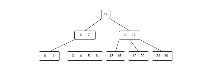
For example, consider a 3-ary tree:
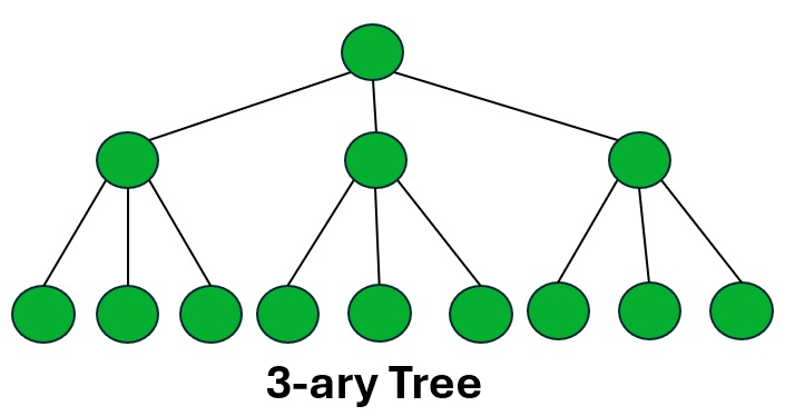
The array representation of the above 3-ary tree is as follows:
The formula to find the parent node of the ith node is (i-1)/3.
The formula to find the child nodes of the ith node is 3*i+1, 3*i+2, 3*i+3.
Array: 1 2 3 4 5 6 7 8 9 10 11 12 13 14 15
Index: 0 1 2 3 4 5 6 7 8 9 10 11 12 13 14

Parent Node:
Parent of 2: (2-1)/3 = 0
Parent of 3: (3-1)/3 = 0
Parent of 4: (4-1)/3 = 1
Parent of 5: (5-1)/3 = 1
Parent of 6: (6-1)/3 = 1
Parent of 7: (7-1)/3 = 2
Parent of 8: (8-1)/3 = 2
Parent of 9: (9-1)/3 = 2
Parent of 10: (10-1)/3 = 3
Parent of 11: (11-1)/3 = 3
Parent of 12: (12-1)/3 = 3
Parent of 13: (13-1)/3 = 4
Parent of 14: (14-1)/3 = 4
Parent of 15: (15-1)/3 = 4
Similarly, we can find the child nodes of each node using the above formula.
Operations on K-Ary Tree
Following are the important operations that can be performed on a K-ary tree:
- Insertion: Insert a new node into the K-ary tree.
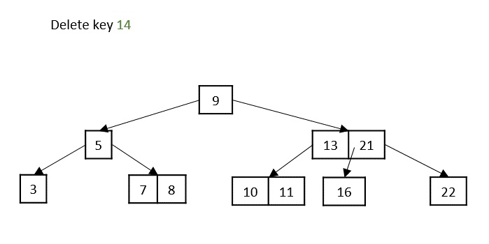
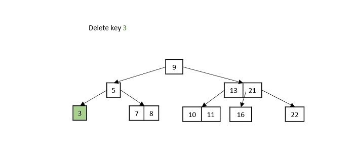
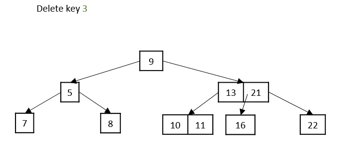
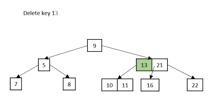
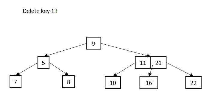
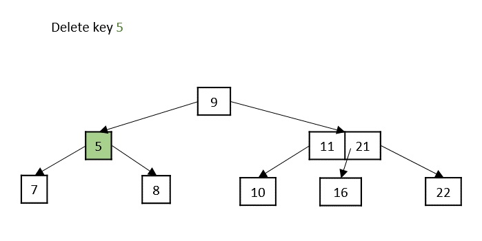
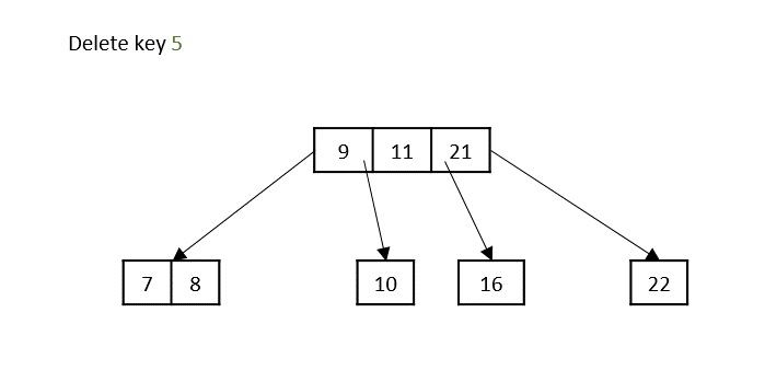
- Deletion: Delete a node from the K-ary tree.
- Traversal: Traverse the K-ary tree in different ways such as inorder, preorder, postorder, and level order.
- Search: Search for a specific node in the K-ary tree.
Implementation of K-Ary Tree
We will discuss the Insertion operation on the K-ary tree. The following is the algorithm to insert a new node into the K-ary tree
Algorithm to Insert a Node in K-Ary Tree
Follow the steps below to insert a new node into the K-ary tree:
1. Create a class Node with data and an array of children.
2. Create a class KaryTree with a root node and a K-ary tree.
3. Insert a new node into the K-ary tree.
Code to Insert a Node in K-Ary Tree
Following is the code to insert a new node into the K-ary tree:
#include <stdio.h>#include <stdlib.h>#define MAX_CHILDREN 3  // Define k (max number of children per node)// Node structure for k-ary treestructNode{int data;structNode* children[MAX_CHILDREN];};// Function to create a new nodestructNode*createNode(int data){structNode* newNode =(structNode*)malloc(sizeof(structNode));
   newNode->data = data;// Initialize all child pointers to NULLfor(int i =0; i < MAX_CHILDREN; i++){
      newNode->children[i]=NULL;}return newNode;}// Function to insert a new child node to a parent nodevoidinsert(structNode* parent,int data){for(int i =0; i < MAX_CHILDREN; i++){if(parent->children[i]==NULL){
         parent->children[i]=createNode(data);return;}}printf("Node %d already has maximum children (%d).\n", parent->data, MAX_CHILDREN);}// Function to print the tree structurevoidprintTree(structNode* root){if(root ==NULL)return;printf("Node %d: ", root->data);for(int i =0; i < MAX_CHILDREN; i++){if(root->children[i]!=NULL){printf("%d ", root->children[i]->data);}}printf("\n");// Recursively print childrenfor(int i =0; i < MAX_CHILDREN; i++){if(root->children[i]!=NULL){printTree(root->children[i]);}}}intmain(){structNode* root =createNode(1);// Insert children into rootinsert(root,2);insert(root,3);insert(root,4);// Insert child nodes into node 3insert(root->children[1],5);insert(root->children[1],6);// Print the tree structureprintTree(root);return0;}
Output
Following is the output of the above C program:
Node 1: 2 3 4
Node 2:
Node 3: 5 6
Node 5:
Node 6:
Node 4:
Traversal of K-Ary Tree
There are different ways to traverse a K-ary tree:
- Inorder Traversal : Traverse the left subtree, visit the root node, and then traverse the right subtree.
- Preorder Traversal : Visit the root node, traverse the left subtree, and then traverse the right subtree.
- Postorder Traversal : Traverse the left subtree, traverse the right subtree, and then visit the root node.
- Level Order Traversal : Traverse the tree level by level from left to right.
Algorithm for Inorder, Preorder, and Postorder Traversal
Follow the steps below to perform an inorder traversal of a K-ary tree:
1. Traverse the left subtree.
2. Visit the root node.
3. Traverse the right subtree.
Follow the steps below to perform a preorder traversal of a K-ary tree:
1. Visit the root node.
2. Traverse the left subtree.
3. Traverse the right subtree.
Follow the steps below to perform a postorder traversal of a K-ary tree:
1. Traverse the left subtree.
2. Traverse the right subtree.
3. Visit the root node.
Code to Perform Inorder, Preorder, and Postorder Traversal
Following is the code to perform inorder, preorder, and postorder traversal of a K-ary tree:
#include <stdio.h>#include <stdlib.h>#define MAX_CHILDREN 3structNode{int data;structNode* children[MAX_CHILDREN];};structNode*createNode(int data){structNode* newNode =(structNode*)malloc(sizeof(structNode));
   newNode->data = data;for(int i =0; i < MAX_CHILDREN; i++){
      newNode->children[i]=NULL;}return newNode;}voidinorder(structNode* root){if(root ==NULL)return;int mid = MAX_CHILDREN /2;// Find the middle index for ordering// First, traverse the left children (half of them)for(int i =0; i < mid; i++){inorder(root->children[i]);}printf("%d ", root->data);// Then, traverse the right children (remaining half)for(int j = mid; j < MAX_CHILDREN; j++){inorder(root->children[j]);}}voidpreorder(structNode* root){if(root ==NULL)return;printf("%d ", root->data);for(int i =0; i < MAX_CHILDREN; i++){preorder(root->children[i]);}}voidpostorder(structNode* root){if(root ==NULL)return;for(int i =0; i < MAX_CHILDREN; i++){postorder(root->children[i]);}printf("%d ", root->data);}intmain(){structNode* root =createNode(1);
   root->children[0]=createNode(2);
   root->children[1]=createNode(3);
   root->children[2]=createNode(4);
   root->children[1]->children[0]=createNode(5);
   root->children[1]->children[1]=createNode(6);printf("Inorder Traversal: ");inorder(root);printf("\n");printf("Preorder Traversal: ");preorder(root);printf("\n");printf("Postorder Traversal: ");postorder(root);printf("\n");return0;}
Output
Following is the output of the above C program:
Inorder Traversal: 2 1 3 5 6 4
Preorder Traversal: 1 2 3 5 6 4
Postorder Traversal: 2 5 6 3 4 1
Level Order Traversal on K-ary Tree
Follow the steps below to perform a level order traversal of a K-ary tree:
1. Create a queue and enqueue the root node.
2. Repeat the following steps until the queue is empty:
   a. Dequeue a node from the queue.
   b. Print the data of the dequeued node.
   c. Enqueue all children of the dequeued node.
Code to Perform Level Order Traversal
Following is the code to perform a level order traversal of a K-ary tree:
#include <stdio.h>#include <stdlib.h>#define MAX_CHILDREN 3structNode{int data;structNode* children[MAX_CHILDREN];};structNode*createNode(int data){structNode* newNode =(structNode*)malloc(sizeof(structNode));
   newNode->data = data;for(int i =0; i < MAX_CHILDREN; i++){
      newNode->children[i]=NULL;}return newNode;}voidlevelOrder(structNode* root){if(root ==NULL)return;structNode* queue[100];int front =0, rear =0;
   queue[rear++]= root;while(front < rear){structNode* current = queue[front++];printf("%d ", current->data);for(int i =0; i < MAX_CHILDREN; i++){if(current->children[i]!=NULL){
            queue[rear++]= current->children[i];}}}}intmain(){structNode* root =createNode(1);
   root->children[0]=createNode(2);
   root->children[1]=createNode(3);
   root->children[2]=createNode(4);
   root->children[1]->children[0]=createNode(5);
   root->children[1]->children[1]=createNode(6);printf("Level Order Traversal: ");levelOrder(root);printf("\n");return0;}
Output
Following is the output of the above C program:
Level Order Traversal: 1 2 3 4 5 6
Search Operation on K-Ary Tree
Follow the steps below to search for a specific node in a K-ary tree:
1. Create a queue and enqueue the root node.
2. Repeat the following steps until the queue is empty:
   a. Dequeue a node from the queue.
   b. If the data of the dequeued node matches the search key, return true.
   c. Enqueue all children of the dequeued node.
3. If the search key is not found, return false.
Code to Search a Node in K-Ary Tree
Following is the code to search for a specific node in a K-ary tree:
#include <stdio.h>#include <stdlib.h>#define MAX_CHILDREN 3structNode{int data;structNode* children[MAX_CHILDREN];};structNode*createNode(int data){structNode* newNode =(structNode*)malloc(sizeof(structNode));
   newNode->data = data;for(int i =0; i < MAX_CHILDREN; i++){
      newNode->children[i]=NULL;}return newNode;}intsearch(structNode* root,int key){if(root ==NULL)return0;structNode* queue[100];int front =0, rear =0;
   queue[rear++]= root;while(front < rear){structNode* current = queue[front++];if(current->data == key)return1;for(int i =0; i < MAX_CHILDREN; i++){if(current->children[i]!=NULL){
            queue[rear++]= current->children[i];}}}return0;}intmain(){structNode* root =createNode(1);
   root->children[0]=createNode(2);
   root->children[1]=createNode(3);
   root->children[2]=createNode(4);
   root->children[1]->children[0]=createNode(5);
   root->children[1]->children[1]=createNode(6);int key =5;if(search(root, key)){printf("Node %d found in the tree.\n", key);}else{printf("Node %d not found in the tree.\n", key);}return0;}
Output
Following is the output of the above C program:
Node 5 found in the tree.
Applications of K-Ary Tree
K-ary tree is used in the following applications:
- File systems
- Routing tables
- Database indexing
- Multiway search trees
- Heap data structure
Conclusion
In this tutorial, we learned about K-ary trees, their representation, and different operations like insertion, traversal, search, and level order traversal. We also discussed the applications of K-ary trees. You can now implement K-ary trees in your programs and solve problems related to them.