Matrix Chain Multiplication is an algorithm that is applied to determine the lowest cost way for multiplying matrices. The actual multiplication is done using the standard way of multiplying the matrices, i.e., it follows the basic rule that the number of rows in one matrix must be equal to the number of columns in another matrix. Hence, multiple scalar multiplications must be done to achieve the product.
To brief it further, consider matrices A, B, C, and D, to be multiplied; hence, the multiplication is done using the standard matrix multiplication. There are multiple combinations of the matrices found while using the standard approach since matrix multiplication is associative. For instance, there are five ways to multiply the four matrices given above −
- (A(B(CD)))
- (A((BC)D))
- ((AB)(CD))
- ((A(BC))D)
- (((AB)C)D)
Now, if the size of matrices A, B, C, and D are l m, m n, n p, p q respectively, then the number of scalar multiplications performed will be lmnpq. But the cost of the matrices change based on the rows and columns present in it. Suppose, the values of l, m, n, p, q are 5, 10, 15, 20, 25 respectively, the cost of (A(B(CD))) is 5 100 25 = 12,500; however, the cost of (A((BC)D)) is 10 25 37 = 9,250.
So, dynamic programming approach of the matrix chain multiplication is adopted in order to find the combination with the lowest cost.
Matrix Chain Multiplication Algorithm
Matrix chain multiplication algorithm is only applied to find the minimum cost way to multiply a sequence of matrices. Therefore, the input taken by the algorithm is the sequence of matrices while the output achieved is the lowest cost parenthesization.
Algorithm
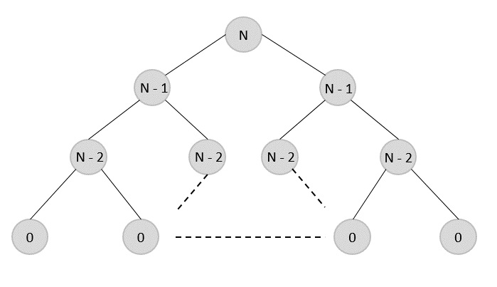
- Count the number of parenthesizations. Find the number of ways in which the input matrices can be multiplied using the formulae −
P(n)={1∑n−1k=1P(k)P(n−k)ifn=1ifn≥2
(or)
P(n)={2(n−1)Cn−1n1ifn≥2ifn=1
- Once the parenthesization is done, the optimal substructure must be devised as the first step of dynamic programming approach so the final product achieved is optimal. In matrix chain multiplication, the optimal substructure is found by dividing the sequence of matrices A[i.j] into two parts A[i,k] and A[k+1,j]. It must be ensured that the parts are divided in such a way that optimal solution is achieved.
- Using the formula, C[i,j]={0mini≤k<j{C[i,k]+C[k+1,j]+di−1dkdjifi=jifi<j find the lowest cost parenthesization of the sequence of matrices by constructing cost tables and corresponding k values table.
- Once the lowest cost is found, print the corresponding parenthesization as the output.
Pseudocode
Pseudocode to find the lowest cost of all the possible parenthesizations −
MATRIX-CHAIN-MULTIPLICATION(p)
   n = p.length  1
   let m[1n, 1n] and s[1n  1, 2n] be new matrices
   for i = 1 to n
      m[i, i] = 0
   for l = 2 to n // l is the chain length
      for i = 1 to n - l + 1
         j = i + l - 1
         m[i, j] = ∞
         for k = i to j - 1
            q = m[i, k] + m[k + 1, j] + pi-1pkpj
            if q < m[i, j]
               m[i, j] = q
               s[i, j] = k
return m and s
Pseudocode to print the optimal output parenthesization −
PRINT-OPTIMAL-OUTPUT(s, i, j )
if i == j
print Ai
else print (
PRINT-OPTIMAL-OUTPUT(s, i, s[i, j])
PRINT-OPTIMAL-OUTPUT(s, s[i, j] + 1, j)
print )
Example
The application of dynamic programming formula is slightly different from the theory; to understand it better let us look at few examples below.
A sequence of matrices A, B, C, D with dimensions 5 10, 10 15, 15 20, 20 25 are set to be multiplied. Find the lowest cost parenthesization to multiply the given matrices using matrix chain multiplication.
Solution
Given matrices and their corresponding dimensions are −
A5×10×B10×15×C15×20×D20×25
Find the count of parenthesization of the 4 matrices, i.e. n = 4.
Using the formula, P(n)={1∑n−1k=1P(k)P(n−k)ifn=1ifn≥2
Since n = 4 2, apply the second case of the formula −
P(n)=∑k=1n−1P(k)P(n−k)
P(4)=∑k=13P(k)P(4−k)
P(4)=P(1)P(3)+P(2)P(2)+P(3)P(1)
If P(1) = 1 and P(2) is also equal to 1, P(4) will be calculated based on the P(3) value. Therefore, P(3) needs to determined first.
P(3)=P(1)P(2)+P(2)P(1)
=1+1=2
Therefore,
P(4)=P(1)P(3)+P(2)P(2)+P(3)P(1)
=2+1+2=5
Among these 5 combinations of parenthesis, the matrix chain multiplicatiion algorithm must find the lowest cost parenthesis.
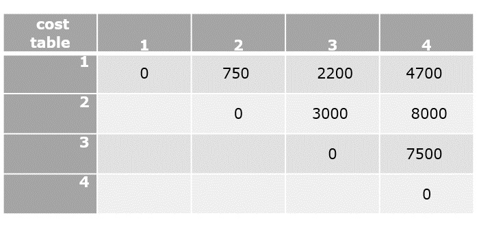
Step 1
The table above is known as a cost table, where all the cost values calculated from the different combinations of parenthesis are stored.
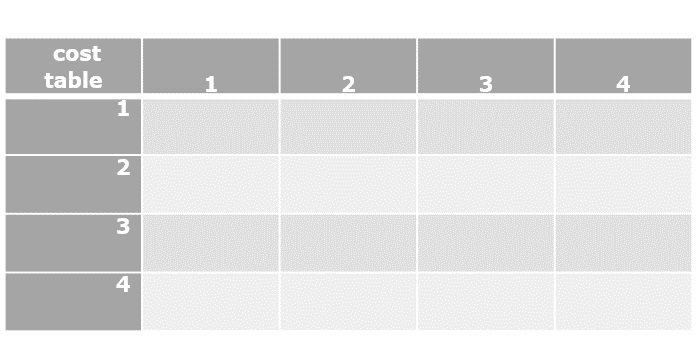
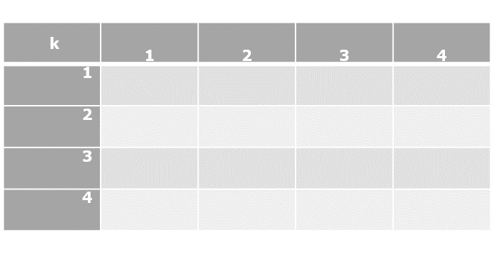
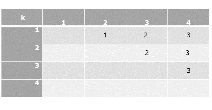
Another table is also created to store the k values obtained at the minimum cost of each combination.
Step 2
Applying the dynamic programming approach formula find the costs of various parenthesizations,
C[i,j]={0mini≤k<j{C[i,k]+C[k+1,j]+di−1dkdjifi=jifi<j
C[1,1]=0
C[2,2]=0
C[3,3]=0
C[4,4]=0

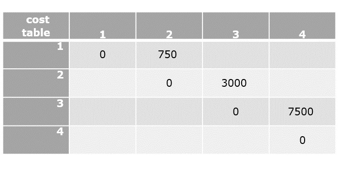
Step 3
Applying the dynamic approach formula only in the upper triangular values of the cost table, since i < j always.
C[1,2]=min1≤k<2{C[1,1]+C[2,2]+d0d1d2}
- C[1,2]=0+0+(5×10×15)
- C[1,2]=750
C[2,3]=min2≤k<3{C[2,2]+C[3,3]+d1d2d3}
- C[2,3]=0+0+(10×15×20)
- C[2,3]=3000
C[3,4]=min3≤k<4{C[3,3]+C[4,4]+d2d3d4}
- C[3,4]=0+0+(15×20×25)
- C[3,4]=7500
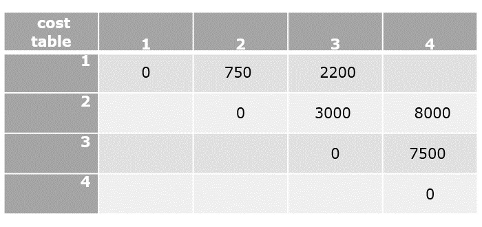
Step 4
Find the values of [1, 3] and [2, 4] in this step. The cost table is always filled diagonally step-wise.
C[2,4]=min2≤k<4{C[2,2]+C[3,4]+d1d2d4,C[2,3]+C[4,4]+d1d3d4}
- C[2,4]=min{(0+7500+(10×15×20)),(3000+5000)}
- C[2,4]=8000
C[1,3]=min1≤k<3{C[1,1]+C[2,3]+d0d1d3,C[1,2]+C[3,3]+d0d2d3}
- C[1,3]=min{(0+3000+1000),(1500+0+750)}
- C[1,3]=2250
Step 5
Now compute the final element of the cost table to compare the lowest cost parenthesization.
C[1,4]=min1≤k<4{C[1,1]+C[2,4]+d0d1d4,C[1,2]+C[3,4]+d1d2d4,C[1,3]+C[4,4]+d1d3d4}
- C[1,4]=min{0+8000+1250,750+7500+1875,2200+0+2500}
- C[1,4]=4700
Now that all the values in cost table are computed, the final step is to parethesize the sequence of matrices. For that, k table needs to be constructed with the minimum value of k corresponding to every parenthesis.
Parenthesization
Based on the lowest cost values from the cost table and their corresponding k values, let us add parenthesis on the sequence of matrices.
The lowest cost value at [1, 4] is achieved when k = 3, therefore, the first parenthesization must be done at 3.
(ABC)(D)
The lowest cost value at [1, 3] is achieved when k = 2, therefore the next parenthesization is done at 2.
((AB)C)(D)
The lowest cost value at [1, 2] is achieved when k = 1, therefore the next parenthesization is done at 1. But the parenthesization needs at least two matrices to be multiplied so we do not divide further.
((AB)(C))(D)
Since, the sequence cannot be parenthesized further, the final solution of matrix chain multiplication is ((AB)C)(D).
Implementation
Following is the final implementation of Matrix Chain Multiplication Algorithm to calculate the minimum number of ways several matrices can be multiplied using dynamic programming −
#include <stdio.h>#include <string.h>#define INT_MAX 999999int mc[50][50];intmin(int a,int b){if(a < b)return a;elsereturn b;}intDynamicProgramming(int c[],int i,int j){if(i == j){return0;}if(mc[i][j]!=-1){return
         mc[i][j];}
   mc[i][j]= INT_MAX;for(int k = i; k < j; k++){
      mc[i][j]=min(mc[i][j],DynamicProgramming(c, i, k)+DynamicProgramming(c, k +1, j)+ c[i -1]* c[k]* c[j]);}return mc[i][j];}intMatrix(int c[],int n){int i =1, j = n -1;returnDynamicProgramming(c, i, j);}intmain(){int arr[]={23,26,27,20};int n =sizeof(arr)/sizeof(arr[0]);memset(mc,-1,sizeof mc);printf("Minimum number of multiplications is: %d",Matrix(arr, n));}
Output
Minimum number of multiplications is: 26000