What is Binary Heap?
Heap or Binary Heap is a special case of balanced binary tree data structure. It is a complete binary tree structure. Means, all levels of the tree are fully filled except possibly for the last level which has all keys as left as possible.
In this structure, the root node is compared to its children, meaning that the root node will be either the smallest or the largest element in the tree. The root node will be the topmost element of all the nodes in the tree.
- Max-Heap: key(a) key(b)
- Min-Heap: key(a) key(b)
Representation of Binary Heap
Binary heap is represented as an array. The root element will be at Arr[0]. For any given node at position i, the left child will be at position 2*i + 1 and the right child at position 2*i + 2.
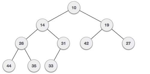
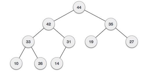
Binary Min-Heap Representation
For a Min-Heap, the root element will be the minimum element in the tree. The left child will be greater than the parent and the right child will be greater than the parent. The representation of a Min-Heap is as follows:
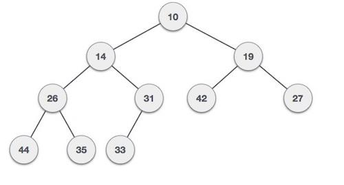
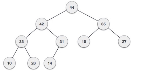
Binary Max-Heap Representation
For a Max-Heap, the root element will be the maximum element in the tree. The left child will be less than the parent and the right child will be less than the parent. The representation of a Max-Heap is as follows:
Operations on Binary Heap
There are mainly three operations that can be performed on a binary heap:
- Insert: Inserting a new element in the heap.
- Delete: Deleting the root element of the heap.
- Peek: Getting the root element of the heap.
Heapify Operation
Heapify operations are used for maintaining the heap property of the binary heap. There are two types of heapify operations:
- Min-Heapify: It is also known as Bubble Down. It is used to maintain the Min-Heap property of the binary heap.
- Max-Heapify: It is also known as Bubble Up. It is used to maintain the Max-Heap property of the binary heap.
Insert Operation on Binary Heap
Inserting a new element in the heap is done by inserting the element at the end of the heap and then heapifying the heap.
The heapifying process is done by comparing the new element with its parent and swapping the elements if the new element is smaller than the parent. The process is repeated until the new element is greater than its parent.
Algorithm for Insert Operation
Following is the algorithm for Insert Operation on Binary Heap:
1.Insert the new element at the end of the heap.
2.Initialize i as the index of the new element.
3.WHILE i is not 0 AND heap[parent(i)] > heap[i]
4.SWAP heap[i] and heap[parent(i)]
5.Update i to parent(i)
Code for Insert Operation
Following is the code for Insert Operation on Binary Heap:
//C Program to perform Insert Operation on Binary Heap#include <stdio.h>intinsert(int heap[],int n,int key){
   n = n +1;int i = n -1;
   heap[i]= key;while(i !=0&& heap[(i-1)/2]> heap[i]){int temp = heap[i];
      heap[i]= heap[(i-1)/2];
      heap[(i-1)/2]= temp;
      i =(i-1)/2;}return n;}intmain(){int heap[100]={10,20,15,40,50,100,25};int n =7;int key =12;
   n =insert(heap, n, key);printf("Heap after Insert Operation: ");for(int i =0; i < n; i++){printf("%d ", heap[i]);}return0;}
Output
Following is the output of the above C program:
Heap after Insert Operation: 10 12 15 20 50 100 25 40
Delete Operation on Binary Heap
Deleting the root element of the heap is done by replacing the root element with the last element of the heap and then heapifying the heap.
The heapifying process is done by comparing the root element with its children and swapping the elements if the root element is greater than its children. The process is repeated until the root element is less than its children.
Algorithm for Delete Operation
Following is the algorithm for Delete Operation on Binary Heap:
START
   Replace the root element with the last element of the heap.
   Initialize i as 0.
   WHILE 2*i + 1 < n
      Set left as 2*i + 1.
      Set right as 2*i + 2.
      Set min as left.
      IF right < n AND heap[right] < heap[left]
         Set min as right.
      IF heap[i] > heap[min]
         SWAP heap[i] and heap[min]
         Update i to min
      ELSE
         BREAK
END
Code for Delete Operation
Following is the code for Delete Operation on Binary Heap:
//C Program to perform Delete Operation on Binary Heap#include <stdio.h>intinsert(int heap[],int n,int key){
   n = n +1;int i = n -1;
   heap[i]= key;while(i !=0&& heap[(i-1)/2]> heap[i]){int temp = heap[i];
      heap[i]= heap[(i-1)/2];
      heap[(i-1)/2]= temp;
      i =(i-1)/2;}return n;}intdelete(int heap[],int n){int root = heap[0];
   heap[0]= heap[n-1];
   n = n -1;int i =0;while(2*i +1< n){int left =2*i +1;int right =2*i +2;int min = left;if(right < n && heap[right]< heap[left]){
         min = right;}if(heap[i]> heap[min]){int temp = heap[i];
         heap[i]= heap[min];
         heap[min]= temp;
         i = min;}else{break;}}return n;}intmain(){int heap[100]={10,20,15,40,50,100,25};int n =7;printf("Heap before Delete Operation: ");for(int i =0; i < n; i++){printf("%d ", heap[i]);}printf("\n");
   n =delete(heap, n);printf("Heap after Delete Operation: ");for(int i =0; i < n; i++){printf("%d ", heap[i]);}return0;}
Output
Following is the output of the above C program:
Heap before Delete Operation: 10 20 15 40 50 100 25
Heap after Delete Operation: 15 20 25 40 50 100
Applications of Binary Heap
Binary Heap is used for many applications. Some of the common applications of Binary Heap are as follows:
- Heap Sort: Heap sort is used to sort an array. It is used in the heap data structure. Binary heap is used to implement heap sort.
- Priority Queue: Binary heap is used for implementing priority queues. It is used in Dijkstra’s algorithm, Prim’s algorithm, etc.
- Graph Algorithms: Binary Heap is used in graph algorithms like Kruskal’s algorithm, Prim’s algorithm, etc.
Conclusion
Binary heaps are useful data structures which can be used to manage the priority of the element. It is the backbone of many algorithms and data structures. It is used in many applications like heap sort, priority queues, graph algorithms, etc.