Approximation algorithms are algorithms designed to solve problems that are not solvable in polynomial time for approximate solutions. These problems are known as NP complete problems. These problems are significantly effective to solve real world problems, therefore, it becomes important to solve them using a different approach.
NP complete problems can still be solved in three cases: the input could be so small that the execution time is reduced, some problems can still be classified into problems that can be solved in polynomial time, or use approximation algorithms to find near-optima solutions for the problems.
This leads to the concept of performance ratios of an approximation problem.
Performance Ratios
The main idea behind calculating the performance ratio of an approximation algorithm, which is also called as an approximation ratio, is to find how close the approximate solution is to the optimal solution.
The approximate ratio is represented using (n) where n is the input size of the algorithm, C is the near-optimal solution obtained by the algorithm, C* is the optimal solution for the problem. The algorithm has an approximate ratio of (n) if and only if −
max{CC∗,C∗C}≤ρ(n)
The algorithm is then called a (n)-approximation algorithm. Approximation Algorithms can be applied on two types of optimization problems: minimization problems and maximization problems. If the optimal solution of the problem is to find the maximum cost, the problem is known as the maximization problem; and if the optimal solution of the problem is to find the minimum cost, then the problem is known as a minimization problem.
For maximization problems, the approximation ratio is calculated by C*/C since 0 C C*. For minimization problems, the approximation ratio is calculated by C/C* since 0 C* C.
Assuming that the costs of approximation algorithms are all positive, the performance ratio is well defined and will not be less than 1. If the value is 1, that means the approximate algorithm generates the exact optimal solution.
Examples
Few popular examples of the approximation algorithms are −
Vertex Cover Algorithm
Set Cover Problem
Travelling Salesman Problem (Approximation Approach)
A Bloom filter is defined as a data structure designed to identify of a elements presence in a set in a rapid and memory efficient manner.
You can think of it as a probabilistic data structure. This data structure helps us to identify that an element is either present or absent in a set. It is not used to store the actual data, but to check whether the data is present or not.
It is a space-efficient probabilistic data structure that is used to test whether an element is a member of a set. False positive matches are possible, but false negatives are not. In other words, a query returns either “possibly in set” or “definitely not in set”.
How Bloom Filter Works?
Let’s understand how a Bloom filter works with the help of an example:
Suppose we have a set of elements {A, B, C, D, E, F, G, H, I, J} and we want to check whether the element ‘X’ is present in the set or not.
Here’s how a Bloom filter works:
Initially, we create a bit array of size ‘m’ and initialize all bits to 0.
We also create ‘k’ hash functions, each of which maps an element to one of the ‘m’ bits.
For each element in the set, we calculate the ‘k’ hash values and set the corresponding bits in the bit array to 1.
When we want to check whether an element ‘X’ is present in the set, we calculate the ‘k’ hash values for ‘X’ and check if all the corresponding bits are set to 1.
If all the bits are set to 1, we say that ‘X’ is possibly in the set. If any of the bits is 0, we say that ‘X’ is definitely not in the set.
Implementation of Bloom Filter
Here’s an example implementation of a Bloom filter C, C++, Java and Python:
A bit mask is a powerful technique that is widely used in computer science and programming to manipulate bits. You can think of it as a way to turn on or off specific bits in a binary number.
Bit masks are used for performing bitwise operations, such as AND, OR, XOR, and NOT, on binary numbers. They are commonly used in computer science for various applications, we will discuss about the bit mask in detail in this chapter.
What is Bit Mask?
Bitmask, also known as mask is a sequence of N-bits that encode the subset of our collection. The element of the mask can be either set or not set (i.e. 0 or 1). This denotes the availability of the chosen element in the bitmask.
For example, an element i is available in the subset if the ith bit of mask is set. For the N element set, there can be a 2N mask each corresponding to a subset.
So, for solving the problem, we will start for a mask i.e. a subset assigns it a value and then finds the values for further masks using the values of the previous mask. Using this we will finally be able to calculate the value of the main set.
Bitwise Operations on Bit Mask
Now, let’s discuss the bitwise operations that can be performed on a bit mask:
AND Operation: The AND operation is used to set a bit to 1 if both bits are 1, otherwise it will be set to 0.
OR Operation: The OR operation is used to set a bit to 1 if either of the bits is 1, otherwise it will be set to 0.
XOR Operation: The XOR operation is used to set a bit to 1 if the bits are different, otherwise it will be set to 0.
NOT Operation: The NOT operation is used to invert the bits, i.e. 1 will be converted to 0 and 0 will be converted to 1.
Operations on Bit Mask
There are mainly three operations that can be performed on a bit mask:
Set: Setting a bit to 1 in a binary number.
Clear: Clearing a bit to 0 in a binary number.
Toggle: Toggling a bit from 0 to 1 or 1 to 0 in a binary number.
Set Operation on Bit Mask
Setting a bit to 1 in a binary number is done by using the OR operation. The OR operation is used to set a bit to 1 if either of the bits is 1, otherwise it will be set to 0.
Algorithm for Set Operation
Following is the algorithm to set the ith bit to 1 in the binary number:
1.Read the binary number and the position of the bit to set.
2.Create a mask with a 1 at the ith position using left shift.
3.Perform the OR operation between the binary number and the mask to set the ith bit.
4.Output the modified binary number.
Code for Set Operation
Here is the code for performing the Set operation on a bit mask in different programming languages:
//C Program to perform Set Operation on Bit Mask#include <stdio.h>intsetBit(int num,int pos){return num |(1<< pos);}intmain(){int num =5;int pos =1;
   num =setBit(num, pos);printf("Number after Set Operation: %d\n", num);return0;}
Output
Number after Set Operation: 7
Clear Operation on Bit Mask
Clearing a bit to 0 in a binary number is done by using the AND operation. The AND operation is used to set a bit to 1 if both bits are 1, otherwise it will be set to 0.
Why do we need to clear a bit to 0?
Sometimes, we need to clear a bit to 0 in a binary number to perform further operations on it. For example, if we want to set a bit to 1, we first clear the bit to 0 and then set it to 1.
Algorithm for Clear Operation
Following is the algorithm to clear the ith bit to 0 in the binary number:
1.Read the binary number and the position of the bit to clear.
2.Create a mask with a 1 at the ith position using left shift and then invert it.
3.Perform the AND operation between the binary number and the mask to clear the ith bit.
4.Output the modified binary number.
Code for Clear Operation
Here is the code for performing the Clear operation on a bit mask in different programming languages:
//C Program to perform Clear Operation on Bit Mask#include <stdio.h>intclearBit(int num,int pos){return num &~(1<< pos);}intmain(){int num =7;int pos =1;
   num =clearBit(num, pos);printf("Number after Clear Operation: %d\n", num);return0;}
Output
Number after Clear Operation: 5
Toggle Operation on Bit Mask
Toggling a bit from 0 to 1 or 1 to 0 in a binary number is done by using the XOR operation. The XOR operation is used to set a bit to 1 if the bits are different, otherwise it will be set to 0.
Algorithm for Toggle Operation
Following is the algorithm to toggle the ith bit in the binary number:
1.Read the binary number and the position of the bit to toggle.
2.Toggle the ith bit in the binary number using XOR operation.
3.Output the modified binary number.
Code for Toggle Operation
Here is the code for performing the Toggle operation on a bit mask in different programming languages:
//C Program to perform Toggle Operation on Bit Mask#include <stdio.h>inttoggleBit(int num,int pos){return num ^(1<< pos);}intmain(){int num =5;int pos =1;
   num =toggleBit(num, pos);printf("Number after Toggle Operation: %d\n", num);return0;}
Output
Number after Toggle Operation: 7
Applications of Bit Mask
Bit masks are used in computer science for various applications, such as:
Setting and clearing bits in a binary number.
Performing bitwise operations on binary numbers.
Encoding and decoding data in a compact form.
Implementing data structures like bit arrays and bitmaps.
Optimizing algorithms and data structures for performance.
Conclusion
Bit masks are useful for manipulating bits in a binary number. They are commonly used in computer science and programming for performing bitwise operations on binary numbers.
Bit masks can be used to set, clear, and toggle bits in a binary number, as well as perform bitwise operations like AND, OR, XOR, and NOT. They are a powerful technique for optimizing algorithms and data structures for performance.
Treaps (pronounced as “trees” and “heaps”) are a data structure that is combination of Binary Search Tree and Heap. It is a binary search tree that is also a heap. We can call it a randomized data structure that maintains a dynamic set of elements, it ensures both the binary search order and the heap order.
Imagine a scenario where you have to organize a bookshelf. You want these book to be in a sorted order, but you also want to keep the books that you read most often at the top. Treaps are the data structure that can help you in this scenario.
Properties of Treaps
Following are the properties of Treaps −
Combined with two major data structures: Binary Search Tree and Heap.
Hence it is BST, keys in left sub-tree are less than the root and keys in right subtree are greater than the root.
Has time complexity of O(log n) for search, insert and delete operations.
Randomized data structure.
It is a balanced binary search tree.
The tree height is O(log n) on average.
Structure of Treaps
Each node in a Treap has two fields:
Key: The key is the value of the node.
Priority: The priority is a random number that is assigned to the node.
The key field is used to maintain the binary search tree property, and the priority field is used to maintain the heap property. The priority of a node is always greater than the priority of its children.
Here is an example of a Treap:
        50
       /  \
     30    70
    /  \   / \
   20  40 60  80
Operations on Treaps
There are many operations that can be performed on Treaps. Some of the major operations are:
Search
Insert
Delete
Implementation of Treaps
Now we will see how to implement Treaps in C, C++, Java and Python.
Algorithm for Inserting a Node in Treaps
1. If the root is NULL, create a new node with the key and priority and return the node.
2. If the key is less than the root, insert in the left subtree.
3. If the key is greater than the root, insert in the right subtree.
4. If the priority of the new node is greater than the priority of the root, rotate the new node with the root.
5. Repeat the process until the new node is inserted.
Code for Implementing Treaps
Now, let’s understand the code for implementing Treaps in C, C++, Java and Python.
For implementing treaps, we need to create a structure for the node and define the functions for inserting and rotating the nodes. After that we can insert the nodes and perform the operations on the treap.
Inorder traversal of the given Treap: 20 30 40 50 60 70 80
Search Operation on Treaps
Searching in a Treap is similar to searching in a Binary Search Tree. We start from the root and compare the key with the root. If the key is less than the root, we move to the left subtree. If the key is greater than the root, we move to the right subtree. We continue this process until we find the key or reach a NULL node.
Algorithm for Searching in Treaps
1. Start from the root.
2. If the root is NULL, return NULL.
3. If the key is equal to the root, return the root.
4. If the key is less than the root, search in the left subtree.
5. If the key is greater than the root, search in the right subtree.
6. Repeat the process until the key is found or NULL is reached.
Code for Searching in Treaps
Now, let’s see the code for searching in Treaps in C, C++, Java and Python.
Deletion in a Treap is similar to deletion in a Binary Search Tree. We first search for the key to be deleted. If the key is found, we delete the node and rearrange the tree to maintain the heap property. We can delete the node by replacing it with the node that has the smallest priority in the right subtree or the node that has the largest priority in the left subtree.
Algorithm for Deleting a Node in Treaps
1. Search for the key to be deleted.
2. If the key is not found, return NULL.
3. If the key is found, delete the node.
4. If the node has no children, delete the node.
5. If the node has one child, replace the node with the child.
6. If the node has two children, replace the node with the node that has the smallest priority in the right subtree or the node that has the largest priority in the left subtree.
7. Repeat the process until the node is deleted.
Code for Deleting a Node in Treaps
Now, let’s see the code for deleting a node in Treaps in C, C++, Java and Python.
Inorder traversal of the given Treap: 20 30 40 50 60 70 80
Inorder traversal of the given Treap after deletion: 30 40 50 60 70 80
Time Complexity of Treaps
Following is the time complexity of Treaps:
Insertion: O(log n) on average.
Deletion: O(log n) on average.
Search: O(log n) on average.
Applications of Treaps
It is used in the implementation of priority queues.
Also used in online algorithms.
Useful in dynamic optimization problems.
Helpful in interval scheduling.
Conclusion
In this chapter, we learned about Treaps, which are a combination of Binary Search Trees and Heaps. We saw the structure of Treaps, the operations that can be performed on Treaps, and the implementation of Treaps in C, C++, Java and Python. We also saw the time and space complexity of Treaps along with the applications of Treaps.
A suffix trie is a type of trie mainly used for representing all the suffixes of a string. It is a tree where each node represents the suffix of a string. The root node is the entire string, and each child node is a suffix of the string that’s one character shorter than the parent node’s suffix.
For example, consider the string “banana”. The suffix trie for this string would look like this:
             root
           /  | \
          b   a  n
         /    |   \
         a    n    a
        /     |     \
        n     a      n
       /      |       \
      a       n        a
     /        |         \
    n         a          $
   /          |
  a           $
 /
$
Each path from the root to a leaf node represents a suffix of the string. The leaf nodes represent the end of a suffix, and the dollar sign ($) is used to indicate the end of the string.
The children store entire word instead of characters.
Features of Suffix Tries
Following are the Features of Suffix Tries −
Operations on Suffix Tries
Some of the common operations on suffix tries include:
Insertion: Insert a new suffix into the trie.
Deletion: Remove a suffix from the trie.
Search: Find a specific suffix in the trie.
Insertion Operation on Suffix Tries
We can insert a new suffix into the trie by following these steps:
1. Start at the root node.
2. For each character in the suffix:
    a. If the character is not in the current node's children, create a new node for the same.
    b. Then move to the child node corresponding to the character and repeat the process.
3. Repeat the process for all character in the suffix.
4. Mark the last node as a leaf node to indicate the end of the suffix.
Code for Insertion Operation
For example, to insert the suffix “ana” into the trie, we would follow these steps:
// C Program to insert a suffix into a trie#include <stdio.h>#include <stdlib.h>#define ALPHABET_SIZE 26// Structure for trie nodestructTrieNode{structTrieNode* children[ALPHABET_SIZE];int isEndOfWord;};// Function to create a new trie nodestructTrieNode*createNode(){structTrieNode* node =(structTrieNode*)malloc(sizeof(structTrieNode));
   node->isEndOfWord =0;for(int i =0; i < ALPHABET_SIZE; i++){
      node->children[i]=NULL;}return node;}// Function to insert a suffix into the trievoidinsert(structTrieNode* root,constchar* suffix){structTrieNode* current = root;for(int i =0; suffix[i]!='\0'; i++){int index = suffix[i]-'a';if(current->children[index]==NULL){
         current->children[index]=createNode();}
      current = current->children[index];}
   current->isEndOfWord =1;}// Display the trievoiddisplay(structTrieNode* root,char str[],int level){if(root->isEndOfWord){
      str[level]='\0';printf("%s\n", str);}for(int i =0; i < ALPHABET_SIZE; i++){if(root->children[i]!=NULL){
         str[level]= i +'a';display(root->children[i], str, level +1);}}}intmain(){structTrieNode* root =createNode();insert(root,"banana");insert(root,"ana");insert(root,"na");insert(root,"a");insert(root,"$");char str[20];// Allocating memory for string bufferdisplay(root, str,0);return0;}
Output
Following is the output of the above code:
a
ana
banana
na
Deletion and Search Operations on Suffix Tries
Deletion and search operations on suffix tries are similar to insertion. We can delete a suffix by removing the corresponding leaf node from the trie. To search for a specific suffix, we can traverse the trie from the root node to the leaf node corresponding to the suffix.
Following are the steps to delete a suffix from the trie:
1. Start at the root node.
2. For each character in the suffix:
    a. Move to the child node corresponding to the character.
3. Mark the last node as a non-leaf node to delete the suffix.
Following are the steps to search for a specific suffix in the trie:
1. Start at the root node.
2. For each character in the suffix:
    a. Move to the child node corresponding to the character.
3. Check if the last node is a leaf node to find the suffix.
Code for Deletion and Search Operations
Here is the code for deletion and search operations on suffix tries:
// C Program to delete and search a suffix in a trie#include <stdio.h>#include <stdlib.h>#define ALPHABET_SIZE 26// Structure for trie nodestructTrieNode{structTrieNode* children[ALPHABET_SIZE];int isEndOfWord;};// Function to create a new trie nodestructTrieNode*createNode(){structTrieNode* node =(structTrieNode*)malloc(sizeof(structTrieNode));
   node->isEndOfWord =0;for(int i =0; i < ALPHABET_SIZE; i++){
      node->children[i]=NULL;}return node;}// Function to insert a suffix into the trievoidinsert(structTrieNode* root,constchar* suffix){structTrieNode* current = root;for(int i =0; suffix[i]!='\0'; i++){int index = suffix[i]-'a';if(current->children[index]==NULL){
         current->children[index]=createNode();}
      current = current->children[index];}
   current->isEndOfWord =1;}// Function to delete a suffix from the trievoiddelete(structTrieNode* root,constchar* suffix){structTrieNode* current = root;for(int i =0; suffix[i]!='\0'; i++){int index = suffix[i]-'a';if(current->children[index]==NULL){return;// Suffix not found}
      current = current->children[index];}
   current->isEndOfWord =0;}// Function to search for a suffix in the trieintsearch(structTrieNode* root,constchar* suffix){structTrieNode* current = root;for(int i =0; suffix[i]!='\0'; i++){int index = suffix[i]-'a';if(current->children[index]==NULL){return0;// Suffix not found}
      current = current->children[index];}return current->isEndOfWord;}intmain(){structTrieNode* root =createNode();insert(root,"banana");insert(root,"ana");insert(root,"na");insert(root,"a");insert(root,"$");printf("Search for 'ana': %s\n",search(root,"ana")?"Found":"Not found");delete(root,"ana");printf("After deletion:\n");printf("Search for 'ana': %s\n",search(root,"ana")?"Found":"Not found");printf("Search for 'na': %s\n",search(root,"na")?"Found":"Not found");return0;}
Output
Following is the output of the above code:
Search for 'ana': Found
After deletion:
Search for 'ana': Not found
Search for 'na': Found
Time Complexity of Suffix Tries
The time complexity of suffix tries depends on the operations performed:
Insertion: O(n) for inserting a suffix of length n into the trie.
Deletion: O(n)
Search: O(n)
Applications of Suffix Tries
Suffix tries are used in various applications, including:
Pattern matching and substring search algorithms
Text indexing and searching
Genomic sequence analysis
Spell checking and correction
Biological sequence analysis
Information retrieval
Compression algorithms
Conclusion
In this chapter, we discussed suffix tries, a type of trie used for representing all the suffixes of a string. We explored the structure of a suffix trie, its features, operations, and applications. Suffix tries are a powerful data structure for substring searches, pattern matching, and other string-related operations.
Compressed Trie is also known as Patricia Trie or Radix Tree. It is a type of trie data structure that is used for storing and retrieving keys in a dataset, where the keys are strings.
You can think of a compressed trie as a trie where the nodes with only one child are merged with their parent nodes. This helps in reducing the space complexity of the trie and makes it more efficient.
The compression of redundant nodes helps in memory management. This type of trie is used with applications that need space management.
Properties of Compressed Tries
Following are some of the properties of compressed tries:
The nodes of compressed tries have at least two children.
The edges of the trie are labeled with characters.
The keys are stored in the leaves of the trie.
Representation of Compressed Tries
Now, let’s see how a compressed trie is represented:
It is represented as a tree where each node has a label and a list of children. The edges of the tree are labeled with characters. The keys are stored in the leaves of the tree.
Here is an example of a compressed trie:
    (root)
      |
     b
     |
    e, i
    |   \
  ar, ll  d
      \    \
       l     l
      /       \
    d, ll    bull
In the above example, the keys “bear”, “bell”, “bid”, “bull” are stored in the leaves of the trie.
Operations on Compressed Tries
We can perform the following operations on compressed tries:
Insert: Inserting a new key into the trie.
Search: Searching for a key in the trie.
Delete: Deleting a key from the trie.
Insert Operation on Compressed Tries
For insertion of a new key into the compressed trie, we need to follow these steps:
Algorithm for Insert Operation
Following is the algorithm for inserting a new key into the compressed trie:
Insert the new key into the trie.
If the node has only one child, merge it with its parent.
Code for Insert Operation
Now, let’s implement the insert operation in a compressed trie. For this, first we need to define the structure of the trie node then implement the insert operation.
//C Program to perform Insert Operation on Compressed Trie#include <stdio.h>#include <stdlib.h>#include <string.h>#define ALPHABET_SIZE 26// Structure for Trie NodestructTrieNode{structTrieNode* children[ALPHABET_SIZE];int isEndOfWord;};// Function to create a new Trie NodestructTrieNode*createNode(){structTrieNode* node =(structTrieNode*)malloc(sizeof(structTrieNode));
   node->isEndOfWord =0;for(int i =0; i < ALPHABET_SIZE; i++){
      node->children[i]=NULL;}return node;}// Function to insert a key into the Trievoidinsert(structTrieNode* root,char* key){structTrieNode* temp = root;for(int i =0; i <strlen(key); i++){int index = key[i]-'a';if(!temp->children[index]){
         temp->children[index]=createNode();}
      temp = temp->children[index];}
   temp->isEndOfWord =1;}voiddisplay(structTrieNode* root,char str[],int level){if(root->isEndOfWord){
      str[level]='\0';printf("%s\n", str);}for(int i =0; i < ALPHABET_SIZE; i++){if(root->children[i]){
         str[level]= i +'a';display(root->children[i], str, level +1);}}}// Main Functionintmain(){structTrieNode* root =createNode();char keys[][8]={"bear","bell","bid","bull"};for(int i =0; i <4; i++){insert(root, keys[i]);}char str[20];display(root, str,0);return0;}
Output
Following is the output of the above code:
bear
bell
bid
bull
Search Operation on Compressed Tries
For searching a key in the compressed trie, we need to follow these steps:
Algorithm for Search Operation
Following is the algorithm for searching a key in the compressed trie:
Search for the key in the trie.
If the key is found, return true.
Otherwise, return false.
Code for Search Operation
Now, let’s implement the search operation in a compressed trie. For this, we need to define the structure of the trie node and then implement the search operation.
//C Program to perform Search Operation on Compressed Trie#include <stdio.h>#include <stdlib.h>#include <string.h>#define ALPHABET_SIZE 26// Structure for Trie NodestructTrieNode{structTrieNode* children[ALPHABET_SIZE];int isEndOfWord;};// Function to create a new Trie NodestructTrieNode*createNode(){structTrieNode* node =(structTrieNode*)malloc(sizeof(structTrieNode));
   node->isEndOfWord =0;for(int i =0; i < ALPHABET_SIZE; i++){
      node->children[i]=NULL;}return node;}// Function to insert a key into the Trievoidinsert(structTrieNode* root,char* key){structTrieNode* temp = root;for(int i =0; i <strlen(key); i++){int index = key[i]-'a';if(!temp->children[index]){
         temp->children[index]=createNode();}
      temp = temp->children[index];}
   temp->isEndOfWord =1;}// Function to search a key in the Trieintsearch(structTrieNode* root,char* key){structTrieNode* temp = root;for(int i =0; i <strlen(key); i++){int index = key[i]-'a';if(!temp->children[index]){return0;}
      temp = temp->children[index];}return(temp !=NULL&& temp->isEndOfWord);}voiddisplay(structTrieNode* root,char str[],int level){if(root->isEndOfWord){
      str[level]='\0';printf("%s\n", str);}for(int i =0; i < ALPHABET_SIZE; i++){if(root->children[i]){
         str[level]= i +'a';display(root->children[i], str, level +1);}}}// Main Functionintmain(){structTrieNode* root =createNode();char keys[][8]={"bear","bell","bid","bull"};for(int i =0; i <4; i++){insert(root, keys[i]);}char str[20];display(root, str,0);char key[]="bell";if(search(root, key)){printf("%s is present in the trie.\n", key);}else{printf("%s is not present in the trie.\n", key);}return0;}
Output
Following is the output of the above code:
bear
bell
bid
bull
bell is present in the trie.
Delete Operation on Compressed Tries
For deleting a key from the compressed trie, we need to follow these steps:
Algorithm for Delete Operation
Following is the algorithm for deleting a key from the compressed trie:
Search for the key in the trie.
If the key is found, mark the last node as not the end of the word.
If the last node has no children, delete it.
Code for Delete Operation
Now, let’s implement the delete operation in a compressed trie. For this, we need to define the structure of the trie node and then implement the delete operation.
//C Program to perform Delete Operation on Compressed Trie#include <stdio.h>#include <stdlib.h>#include <string.h>#define ALPHABET_SIZE 26// Structure for Trie NodestructTrieNode{structTrieNode* children[ALPHABET_SIZE];int isEndOfWord;};// Function to create a new Trie NodestructTrieNode*createNode(){structTrieNode* node =(structTrieNode*)malloc(sizeof(structTrieNode));
   node->isEndOfWord =0;for(int i =0; i < ALPHABET_SIZE; i++){
      node->children[i]=NULL;}return node;}// Function to insert a key into the Trievoidinsert(structTrieNode* root,char* key){structTrieNode* temp = root;for(int i =0; i <strlen(key); i++){int index = key[i]-'a';if(!temp->children[index]){
         temp->children[index]=createNode();}
      temp = temp->children[index];}
   temp->isEndOfWord =1;}// Function to search a key in the Trieintsearch(structTrieNode* root,char* key){structTrieNode* temp = root;for(int i =0; i <strlen(key); i++){int index = key[i]-'a';if(!temp->children[index]){return0;}
      temp = temp->children[index];}return(temp !=NULL&& temp->isEndOfWord);}// Function to delete a key from the Trievoiddelete(structTrieNode* root,char* key){if(!search(root, key)){return;}structTrieNode* temp = root;for(int i =0; i <strlen(key); i++){int index = key[i]-'a';
      temp = temp->children[index];}
   temp->isEndOfWord =0;}voiddisplay(structTrieNode* root,char str[],int level){if(root->isEndOfWord){
      str[level]='\0';printf("%s\n", str);}for(int i =0; i < ALPHABET_SIZE; i++){if(root->children[i]){
         str[level]= i +'a';display(root->children[i], str, level +1);}}}// Main Functionintmain(){structTrieNode* root =createNode();char keys[][8]={"bear","bell","bid","bull"};for(int i =0; i <4; i++){insert(root, keys[i]);}char str[20];display(root, str,0);char key[]="bell";delete(root, key);printf("Trie after deletion:\n");display(root, str,0);if(search(root, key)){printf("%s is present in the trie.\n", key);}else{printf("%s is not present in the trie.\n", key);}return0;}
Output
Following is the output of the above code:
bear
bell
bid
bull
bell is not present in the trie.
Applications of Compressed Tries
Compressed tries are used in various applications, such as:
Spell checkers: In spell checkers, compressed tries are used to store the dictionary of words.
Text editors
Routing tables in computer networks
Genome sequence analysis
String matching algorithms
Conclusion
In this chapter, we learned about compressed tries, which are used to store a large number of strings efficiently. We discussed the structure of a compressed trie, the insert operation, search operation, and delete operation on a compressed trie. We also implemented these operations in C, C++, Java, and Python programming languages.
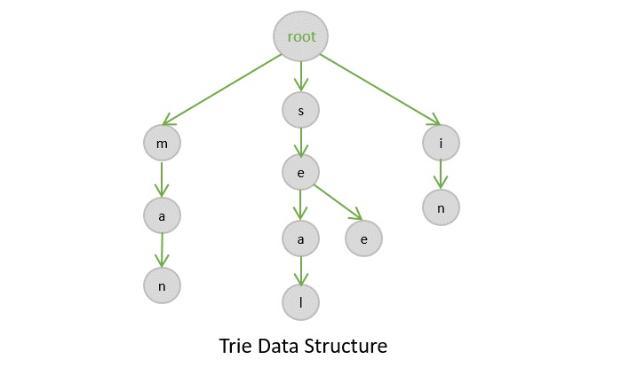
Tries are tree-like data structures that are mainly used for storing dynamic set of strings or associative arrays where the keys are usually strings. The word “trie” comes from the word “retrieval”.
We already discussed the basic concepts of tries in Tries chapter. In this chapter, we will discuss the standard tries in data structures.
What is Standard Trie?
Children of a node are stored in a certain order such as dictionary order (alphabetical) or ASCII order. The order des on the use cases. For example, if the trie is used for a dictionary, the children are stored in alphabetical order.
Let’s understand with an example.
We have an array of Strings.
{cat, car, dog, doll}
The structure of the trie for these strings would be
                   (root)
             	    /\
             	   /  \
             	  /    \
                  /      \
                 c        d
                / \      / \
               a   a    o   o
              /    \   /     \
             t      r l       g
                   /
                  l
The above example shows the standard trie structure for the strings {cat, car, dog, doll}. The root node is empty and the children are stored in alphabetical order.
In the Standard Trie, a string can be traced from the root node to the node where the strings. The node is marked as a leaf node.
Operations on Standard Trie
There are mainly three operations that can be performed on a standard trie:
Insert: Inserting a new string in the trie.
Search: Searching a string in the trie.
Delete: Deleting a string from the trie.
Implementation of Standard Trie
For implementing the standard trie, we need to create a structure for the trie node. The trie node contains an array of pointers to the children nodes and a flag to mark the of the string.
Now, let’s implement the standard trie, which supports the above operations.
Insert Operation on Standard Trie
Inserting a new string in the Standard Trie is done by inserting the characters of the string one by one. The characters are inserted in the trie in the order of the string. The last character of the string is marked as a leaf node.
Algorithm for Insert Operation in Standard Trie
Following is the algorithm for the insert operation in the standard trie:
1.Traverse the trie from the root node.
2.Insert the characters of the string one by one.
3.Mark the last character of the string as a leaf node.
Code for Insert Operation in Standard Trie
Let’s see the code for the insert operation in the standard trie using C, C++, Java, and Python programming languages.
// C Program to perform Insert Operation in Standard Trie#include <stdio.h>#include <stdlib.h>#define ALPHABET_SIZE 26// Structure for Trie NodestructTrieNode{structTrieNode*children[ALPHABET_SIZE];int iOfWord;};// Function to create a new Trie NodestructTrieNode*createNode(){structTrieNode*newNode =(structTrieNode*)malloc(sizeof(structTrieNode));
   newNode->iOfWord =0;for(int i =0; i < ALPHABET_SIZE; i++){
      newNode->children[i]=NULL;}return newNode;}// Function to insert a string in the Trievoidinsert(structTrieNode*root,char*key){structTrieNode*temp = root;for(int i =0; key[i]!='\0'; i++){int index = key[i]-'a';if(!temp->children[index]){
         temp->children[index]=createNode();}
      temp = temp->children[index];}
   temp->iOfWord =1;}voiddisplay(structTrieNode*root,char str[],int level){if(root->iOfWord){
      str[level]='\0';printf("%s\n", str);}for(int i =0; i < ALPHABET_SIZE; i++){if(root->children[i]){
         str[level]= i +'a';display(root->children[i], str, level +1);}}}// Main functionintmain(){char*keys[]={"cat","car","dog","doll"};int n =sizeof(keys)/sizeof(keys[0]);structTrieNode*root =createNode();for(int i =0; i < n; i++){insert(root, keys[i]);}printf("Inserted Strings are:\n");char str[26];display(root, str,0);return0;}
Output
Following is the output obtained −
Inserted Strings are:
car
cat
dog
doll
Search Operation on Standard Trie
Searching a string in the Standard Trie is done by traversing the trie from the root node to the node where the strings. If the string is found in the trie, then the search operation returns true; otherwise, it returns false.
Algorithm for Search Operation in Standard Trie
Following is the algorithm for the search operation in the Standard Trie:
1.Traverse the trie from the root node.
2.Search the characters of the string one by one.
3.If the string is found, return true.
4.If the string is not found, return false.
Code for Search Operation in Standard Trie
Following is the code for the search operation in the Standard Trie using C, C++, Java, and Python programming languages.
// C Program to perform Search Operation in Standard Trie#include <stdio.h>#include <stdlib.h>#define ALPHABET_SIZE 26// Structure for Trie NodestructTrieNode{structTrieNode*children[ALPHABET_SIZE];int iOfWord;};// Function to create a new Trie NodestructTrieNode*createNode(){structTrieNode*newNode =(structTrieNode*)malloc(sizeof(structTrieNode));
   newNode->iOfWord =0;for(int i =0; i < ALPHABET_SIZE; i++){
      newNode->children[i]=NULL;}return newNode;}// Function to insert a string in the Standard Trievoidinsert(structTrieNode*root,char*key){structTrieNode*temp = root;for(int i =0; key[i]!='\0'; i++){int index = key[i]-'a';if(!temp->children[index]){
         temp->children[index]=createNode();}
      temp = temp->children[index];}
   temp->iOfWord =1;}// Function to search a string in the Standard Trieintsearch(structTrieNode*root,char*key){structTrieNode*temp = root;for(int i =0; key[i]!='\0'; i++){int index = key[i]-'a';if(!temp->children[index]){return0;}
      temp = temp->children[index];}return temp !=NULL&& temp->iOfWord;}intmain(){char*keys[]={"cat","car","dog","doll"};int n =sizeof(keys)/sizeof(keys[0]);structTrieNode*root =createNode();for(int i =0; i < n; i++){insert(root, keys[i]);}search(root,"cat")?printf("Found\n"):printf("Not Found\n");return0;}
Output
The output obtained is as follows −
Found
Delete Operation on Standard Trie
Deleting a string from the Standard Trie is done by deleting the characters of the string one by one. The characters are deleted in the order of the string. The last character of the string is marked as a non-leaf node.
Algorithm for Delete Operation in Standard Trie
Following is the algorithm for the delete operation in the Standard Trie:
1.Traverse the trie from the root node.
2.Delete the characters of the string one by one.
3.Mark the last character of the string as a non-leaf node.
Code for Delete Operation in Standard Trie
Let’s see the code for the delete operation in the Standard Trie using C, C++, Java, and Python programming languages.
// C Program to perform Delete Operation in Standard Trie#include <stdio.h>#include <stdlib.h>#define ALPHABET_SIZE 26structTrieNode{structTrieNode*children[ALPHABET_SIZE];int iOfWord;};structTrieNode*createNode(){structTrieNode*newNode =(structTrieNode*)malloc(sizeof(structTrieNode));
   newNode->iOfWord =0;for(int i =0; i < ALPHABET_SIZE; i++){
      newNode->children[i]=NULL;}return newNode;}voidinsert(structTrieNode*root,char*key){structTrieNode*temp = root;for(int i =0; key[i]!='\0'; i++){int index = key[i]-'a';if(!temp->children[index]){
         temp->children[index]=createNode();}
      temp = temp->children[index];}
   temp->iOfWord =1;}intdelete(structTrieNode*root,char*key,int depth){if(root ==NULL){return0;}if(key[depth]=='\0'){if(root->iOfWord){
         root->iOfWord =0;}for(int i =0; i < ALPHABET_SIZE; i++){if(root->children[i]){return0;}}free(root);return1;}int index = key[depth]-'a';if(delete(root->children[index], key, depth +1)){
      root->children[index]=NULL;if(!root->iOfWord){for(int i =0; i < ALPHABET_SIZE; i++){if(root->children[i]){return0;}}free(root);return1;}}return0;}voiddisplay(structTrieNode*root,char str[],int level){if(root ==NULL){return;}if(root->iOfWord){
      str[level]='\0';printf("%s\n", str);}for(int i =0; i < ALPHABET_SIZE; i++){if(root->children[i]){
         str[level]= i +'a';display(root->children[i], str, level +1);}}}intmain(){char*keys[]={"cat","car","dog","doll"};int n =sizeof(keys)/sizeof(keys[0]);structTrieNode*root =createNode();for(int i =0; i < n; i++){insert(root, keys[i]);}printf("Before Deletion:\n");char str[20];display(root, str,0);delete(root,"car",0);printf("\nAfter Deletion:\n");display(root, str,0);return0;}
Output
The output obtained is as follows −
Before Deletion:
car
cat
dog
doll

After Deletion:
cat
dog
doll
Time Complexity of Standard Trie
Following is the time complexity of the Standard Trie:
Insert Operation: O(n), where n is the length of the string.
Search Operation: O(n).
Delete Operation: O(n).
Applications of Standard Trie
Standard Trie is used in various applications such as:
Spell Checker
Auto-Complete
Dictionary
IP Routing
Network Routing
Prefix Matching
These are some of the applications where Standard Trie is used.
Conclusion
In this chapter, we discussed the Standard Trie in data structures. The structure of the Standard Trie, the operations that can be performed on the Standard Trie, and the implementation of the Standard Trie. We also discussed the applications of the Standard Trie.
A trie is a type of a multi-way search tree, which is fundamentally used to retrieve specific keys from a string or a set of strings. It stores the data in an ordered efficient way since it uses pointers to every letter within the alphabet.
The trie data structure works based on the common prefixes of strings. The root node can have any number of nodes considering the amount of strings present in the set. The root of a trie does not contain any value except the pointers to its child nodes.
There are three types of trie data structures −
Standard Tries
Compressed Tries
Suffix Tries
The real-world applications of trie include − autocorrect, text prediction, sentiment analysis and data sciences.
Basic Operations in Tries
The trie data structures also perform the same operations that tree data structures perform. They are −
Insertion
Deletion
Search
Insertion operation
The insertion operation in a trie is a simple approach. The root in a trie does not hold any value and the insertion starts from the immediate child nodes of the root, which act like a key to their child nodes. However, we observe that each node in a trie represents a singlecharacter in the input string. Hence the characters are added into the tries one by one while the links in the trie act as pointers to the next level nodes.
Example
Following are the implementations of this operation in various programming languages −
#include <stdio.h>#include <stdlib.h>#include <string.h>#define ALPHABET_SIZE 26structTrieNode{structTrieNode* children[ALPHABET_SIZE];int isEndOfWord;};structTrie{structTrieNode* root;};structTrieNode*createNode(){structTrieNode* node =(structTrieNode*)malloc(sizeof(structTrieNode));
    node->isEndOfWord =0;for(int i =0; i < ALPHABET_SIZE; i++){
        node->children[i]=NULL;}return node;}voidinsert(structTrie* trie,constchar* key){structTrieNode* curr = trie->root;for(int i =0; i <strlen(key); i++){int index = key[i]-'a';if(curr->children[index]==NULL){
            curr->children[index]=createNode();}
        curr = curr->children[index];}
    curr->isEndOfWord =1;}voidprintWords(structTrieNode* node,char* prefix){if(node->isEndOfWord){printf("%s\n", prefix);}for(int i =0; i < ALPHABET_SIZE; i++){if(node->children[i]!=NULL){char* newPrefix =(char*)malloc(strlen(prefix)+2);strcpy(newPrefix, prefix);
            newPrefix[strlen(prefix)]='A'+ i;
            newPrefix[strlen(prefix)+1]='\0';printWords(node->children[i], newPrefix);free(newPrefix);}}}intmain(){structTrie car;
    car.root =createNode();insert(&car,"lamborghini");insert(&car,"mercedes-Benz");insert(&car,"land Rover");insert(&car,"maruti Suzuki");printf("Trie elements are:\n");printWords(car.root,"");return0;}
Output
Trie elements are:
LAMBORGHINI
LANDNOVER
MARUTIOUZUKI
MERCEZENZ
Deletion operation
The deletion operation in a trie is performed using the bottom-up approach. The element is searched for in a trie and deleted, if found. However, there are some special scenarios that need to be kept in mind while performing the deletion operation.
Case 1 − The key is unique − in this case, the entire key path is deleted from the node. (Unique key suggests that there is no other path that branches out from one path).
Case 2 − The key is not unique − the leaf nodes are updated. For example, if the key to be deleted is see but it is a prefix of another key seethe; we delete the see and change the Boolean values of t, h and e as false.
Case 3 − The key to be deleted already has a prefix − the values until the prefix are deleted and the prefix remains in the tree. For example, if the key to be deleted is heart but there is another key present he; so we delete a, r, and t until only he remains.
Example
Following are the implementations of this operation in various programming languages −
//C code for Deletion Operation of tries Algorithm#include <stdio.h>#include <stdlib.h>#include <stdbool.h>#include <string.h>//Define size 26#define ALPHABET_SIZE 26structTrieNode{structTrieNode* children[ALPHABET_SIZE];
   bool isEndOfWord;};structTrie{structTrieNode* root;};structTrieNode*createNode(){structTrieNode* node =(structTrieNode*)malloc(sizeof(structTrieNode));
   node->isEndOfWord = false;for(int i =0; i < ALPHABET_SIZE; i++){
      node->children[i]=NULL;}return node;}voidinsert(structTrie* trie,constchar* key){structTrieNode* curr = trie->root;for(int i =0; i <strlen(key); i++){int index = key[i]-'a';if(curr->children[index]==NULL){
            curr->children[index]=createNode();}
        curr = curr->children[index];}
    curr->isEndOfWord =1;}
bool search(structTrieNode* root,char* word){structTrieNode* curr = root;for(int i =0; word[i]!='\0'; i++){int index = word[i]-'a';if(curr->children[index]==NULL){return false;}
      curr = curr->children[index];}return(curr !=NULL&& curr->isEndOfWord);}
bool startsWith(structTrieNode* root,char* prefix){structTrieNode* curr = root;for(int i =0; prefix[i]!='\0'; i++){int index = prefix[i]-'a';if(curr->children[index]==NULL){return false;}
      curr = curr->children[index];}return true;}
bool deleteWord(structTrieNode* root,char* word){structTrieNode* curr = root;structTrieNode* parent =NULL;int index;for(int i =0; word[i]!='\0'; i++){
      index = word[i]-'a';if(curr->children[index]==NULL){return false;// Word does not exist in the Trie}
      parent = curr;
      curr = curr->children[index];}if(!curr->isEndOfWord){return false;// Word does not exist in the Trie}
   curr->isEndOfWord = false;// Mark as deletedif(parent !=NULL){
      parent->children[index]=NULL;// Remove the child node}return true;}voidprintWords(structTrieNode* node,char* prefix){if(node->isEndOfWord){printf("%s\n", prefix);}for(int i =0; i < ALPHABET_SIZE; i++){if(node->children[i]!=NULL){char* newPrefix =(char*)malloc(strlen(prefix)+2);strcpy(newPrefix, prefix);
            newPrefix[strlen(prefix)]='a'+ i;
            newPrefix[strlen(prefix)+1]='\0';printWords(node->children[i], newPrefix);free(newPrefix);}}}intmain(){structTrie car;
    car.root =createNode();insert(&car,"lamborghini");insert(&car,"mercedes-Benz");insert(&car,"landrover");insert(&car,"maruti Suzuki");//Before Deletionprintf("Tries elements before deletion: \n");printWords(car.root,"");//Deleting the elementschar* s1  ="lamborghini";char* s2 ="landrover";printf("Elements to be deleted are: %s and %s", s1, s2);deleteWord(car.root, s1);deleteWord(car.root, s2);//After Deletionprintf("\nTries elements before deletion: \n");printWords(car.root,"");}
Output
Tries elements before deletion:
lamborghini
landrover
marutiouzuki
mercezenz
Elements to be deleted are: lamborghini and landrover
Tries elements before deletion:
marutiouzuki
mercezenz
Search operation
Searching in a trie is a rather straightforward approach. We can only move down the levels of trie based on the key node (the nodes where insertion operation starts at). Searching is done until the end of the path is reached. If the element is found, search is successful; otherwise, search is prompted unsuccessful.
Example
Following are the implementations of this operation in various programming languages −
//C program for search operation of tries algorithm#include <stdio.h>#include <stdlib.h>#include <stdbool.h>#define ALPHABET_SIZE 26structTrieNode{structTrieNode* children[ALPHABET_SIZE];
   bool isEndOfWord;};structTrieNode*createNode(){structTrieNode* node =(structTrieNode*)malloc(sizeof(structTrieNode));
   node->isEndOfWord = false;for(int i =0; i < ALPHABET_SIZE; i++){
      node->children[i]=NULL;}return node;}voidinsert(structTrieNode* root,char* word){structTrieNode* curr = root;for(int i =0; word[i]!='\0'; i++){int index = word[i]-'a';if(curr->children[index]==NULL){
         curr->children[index]=createNode();}
      curr = curr->children[index];}
   curr->isEndOfWord = true;}
bool search(structTrieNode* root,char* word){structTrieNode* curr = root;for(int i =0; word[i]!='\0'; i++){int index = word[i]-'a';if(curr->children[index]==NULL){return false;}
      curr = curr->children[index];}return(curr !=NULL&& curr->isEndOfWord);}
bool startsWith(structTrieNode* root,char* prefix){structTrieNode* curr = root;for(int i =0; prefix[i]!='\0'; i++){int index = prefix[i]-'a';if(curr->children[index]==NULL){return false;}
      curr = curr->children[index];}return true;}intmain(){structTrieNode* root =createNode();//inserting the elementsinsert(root,"Lamborghini");insert(root,"Mercedes-Benz");insert(root,"Land Rover");insert(root,"Maruti Suzuki");//Searching elementsprintf("Searching Cars\n");//Printing searched elementsprintf("Found? %d\n",search(root,"Lamborghini"));// Output: 1 (true)printf("Found? %d\n",search(root,"Mercedes-Benz"));// Output: 1 (true)printf("Found? %d\n",search(root,"Honda"));// Output: 0 (false)printf("Found? %d\n",search(root,"Land Rover"));// Output: 1 (true)printf("Found? %d\n",search(root,"BMW"));// Output: 0 (false)   //Searching the elements the name starts with?printf("Cars name starts with\n");//Printing the elementsprintf("Does car name starts with 'Lambo'? %d\n",startsWith(root,"Lambo"));// Output: 1 (true)printf("Does car name starts with 'Hon'? %d\n",startsWith(root,"Hon"));// Output: 0 (false)printf("Does car name starts with 'Hy'? %d\n",startsWith(root,"Hy"));// Output: 0 (false)printf("Does car name starts with 'Mar'? %d\n",startsWith(root,"Mar"));// Output: 1 (true)printf("Does car name starts with 'Land'? %d\n",startsWith(root,"Land"));// Output: 1 (true)   return0;}
Output
Searching Cars
Found? 1
Found? 1
Found? 0
Found? 1
Found? 0
Cars name starts with
Does car name starts with 'Lambo'? 1
Does car name starts with 'Hon'? 0
Does car name starts with 'Hy'? 0
Does car name starts with 'Mar'? 1
Does car name starts with 'Land'? 1
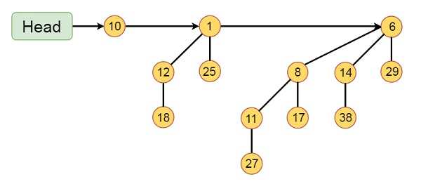
Like Binomial heaps, Fibonacci heaps are collection of trees. They are loosely based on binomial heaps. Unlike trees within binomial heaps, trees within Fibonacci heaps are rooted but unordered.
Each node x in Fibonacci heaps contains a pointer p[x] to its parent, and a pointer child[x] to any one of its children. The children of x are linked together in a circular doubly linked list known as the child list of x.
Each child y in a child list has pointers left[y] and right[y] to point to the left and right siblings of y respectively. If node y is the only child, then left[y] = right[y] = y. The order in which siblings appear in a child list is arbitrary.
Structure of Fibonacci Heap
Each node x in Fibonacci heap contains the following fields:
key[x]: key of node x
degree[x]: number of children of x
p[x]: parent of x
child[x]: any one of the children of x
left[x]: left sibling of x in the child list of x
right[x]: right sibling of x in the child list of x
mark[x]: boolean value to indicate whether x has lost a child since the last time x was made the child of another node
Each Fibonacci heap H is a set of rooted trees that are min-heap ordered. That is, each tree obeys the min-heap property: the key of a node is greater than or equal to the key of its parent.
The root list of H is a circular doubly linked list of elements of H containing exactly one root from each tree in the root list. The min pointer in H points to the root of the tree containing the minimum key.
This Fibonacci Heap H consists of five Fibonacci Heaps and 16 nodes. The line with arrow head indicates the root list. Minimum node in the list is denoted by min[H] which is holding 4.
The asymptotically fast algorithms for problems such as computing minimum spanning trees, finding single source of shortest paths etc. make essential use of Fibonacci heaps.
Operations on Fibonacci Heap
Following are the operations that can be performed on Fibonacci heap:
Make-Fib-Heap().
Fib-Heap-Insert(H, x).
Fib-Heap-Extract-Min(H).
Fib-Heap-Decrease-Key(H, x, k).
Fib-Heap-Delete(H, x).
Insert Operation on Fibonacci Heap
Adds a new node x to the heap H. Its super fast, just inserts without much rearranging.
Algorithm for Insert Operation
Let’s assume that we have a Fibonacci heap H and a node x. The algorithm to insert node x into Fibonacci heap H is as follows:
1: Create a new Fibonacci Heap H' containing only x.
2: Set x.left = x and x.right = x (circular doubly linked list).
3: If H is empty, set H.min = x.
4: Otherwise, Insert x into the root list of H and update H.min if x.key < H.min.key.
5: Increase the total node count of H.
Code for Insert Operation
Let’s write a simple code to insert a node into Fibonacci heap.
Fibonacci Heap Root List: 3 7 10 15
Minimum value in heap: 3
Extract Minimum Operation on Fibonacci Heap
Removes the node containing the minimum key from the heap H. Its a bit complex operation as it involves rearranging the tree structure.
Algorithm
Let’s assume that we have a Fibonacci heap H. The algorithm to extract minimum node from Fibonacci heap H is as follows:
1: z = H.min
2: If z != NULL
   1 - For each child x of z, add x to the root list of H.
   2 - Remove z from the root list of H.
   3 - If z = z.right, then H.min = NULL.
   4 - Else, H.min = z.right and Consolidate(H).
   5 - Decrease the total node count of H.
3: Return z.
Code for Extract Minimum Operation
Let’s write a simple code to extract minimum node from Fibonacci heap.
Decreases the key of node x to the new key k. Its a bit complex operation as it involves rearranging the tree structure.
Algorithm for Decrease Key Operation
Let’s assume that we have a Fibonacci heap H, a node x and a new key k. The algorithm to decrease key of node x to k in Fibonacci heap H is as follows:
1: x.key = k
2: y = x.parent
3: If y != NULL and x.key < y.key
   1 - Cut x from its parent y.
   2 - Cascading-Cut(H, y).
4: If x.key < H.min.key, set H.min = x.
Code for Decrease Key Operation
Let’s write a simple code to decrease key of a node in Fibonacci heap.
Let’s analyze the time complexity of various operations in Fibonacci heap:
Insert Operation: O(1)
Extract Minimum Operation: O(log n)
Decrease Key Operation: O(1)
Delete Operation: O(log n)
Thus, the Fibonacci heap is a data structure that supports insert, extract minimum, decrease key, and delete operations in amortized O(log n) time complexity.
Applications of Fibonacci Heap
Following are some of the applications of Fibonacci heap:
It is used in Dijkstra’s algorithm to find the shortest path in a graph.
Also, used in Prim’s algorithm to find the minimum spanning tree of a graph.
Used in network routing algorithms.
Conclusion
In this tutorial, we learned about Fibonacci heap, its operations, and its time complexity. We also implemented the Fibonacci heap in C, C++, Java, and Python programming languages. We also discussed the applications of Fibonacci heap in various algorithms.
A binomial Heap is a collection of Binomial Trees. A binomial tree Bk is an ordered tree defined recursively. A binomial Tree B0 consists of a single node.
A binomial tree is an ordered tree defined recursively. A binomial tree Bk consists of two binomial trees Bk-1 that are linked together. The root of one is the leftmost child of the root of the other.
Binomial trees are defined recursively. A binomial tree Bk is defined as follows
B0 is a single node.
Bk is formed by linking two binomial trees Bk-1 such that the root of one is the leftmost child of the root of the other.
Some properties of binomial trees are
Binomial tree with Bk has 2k nodes.
Height of the tree is k
There are exactly j! / (i! * (j-i)!) nodes at depth i for all i in range 0 to k.
What is Binomial Heap?
As mentioned above, a binomial heap is a collection of binomial trees. These binomial trees are linked together in a specific way. The binomial heap has the following properties
Each binomial tree in the heap follows the min-heap property.
No two binomial trees in the heap can have the same number of nodes.
There is at most one binomial tree of any order.
Representation of Binomial Heap
Following is a representation of binomial heap, where Bk is a binomial heap of order k.
Some binomial heaps are like below
Example of Binomial Heap
This binomial Heap H consists of binomial trees B0, B2 and B3. Which have 1, 4 and 8 nodes respectively. And in total n = 13 nodes. The root of binomial trees are linked by a linked list in order of increasing degree
Operations on Binomial Heap
Following are the operations that can be performed on a binomial heap
Insert: As name suggests, it is used to insert a node into the heap.
Union: It is used to merge two binomial heaps into a single binomial heap.
Extract-Min: This operation removes the node with the smallest key from the heap.
Decrease-Key: This operation decreases the key of a node in the heap.
Delete: Simply put, it deletes a node from the heap.
Implementation of Binomial Heap
We can implement a binomial heap using a linked list of binomial trees. Each node in the linked list is a binomial tree. The root of each binomial tree is the head of the linked list. The linked list is ordered by the order of the binomial trees. The binomial heap is the head of the linked list.
Implementation of binomial heap using following steps
1. Create a new node with the given key.
2. Merge the new node with the binomial heap.
3. Adjust the binomial heap to maintain the heap property.
4. Insert the new node into the binomial heap.
5. Print the binomial heap.
Code for Binomial Heap
Following is the implementation of binomial heap in C, C++, Java and Python.
In the following code, first we create a structure Node to represent a node in the binomial heap. The structure contains the data, degree, child, sibling, and parent of the node. We then define functions to create a new node, merge two binomial trees, union two binomial heaps, adjust the heap, and insert a new node into the heap. Finally, we print the binomial heap.
The extract-min operation removes the node with the smallest key from the binomial heap. The extract-min operation is performed as follows
1. Find the node with the smallest key in the binomial heap.
2. Remove the node from the binomial heap.
3. Now, Let's Merge the children of the node with the binomial heap.
4. Adjust the binomial heap to maintain the heap property.
5. Return the new binomial heap.
Code for Extract-Min Operation
Following is the implementation of extract-min operation in C, C++, Java and Python.
Decrease-key is a important operation in the binomial heap. It is used to decrease the value of a key in the binomial heap. The decrease-key operation is performed as follows
Algorithm for Decrease-Key Operation
Follow the steps below to decrease-key.
1. Decrease the value of the key to a new value.
2. If the new value is greater than the parent of the node, then return.
3. If the new value is less than the parent of the node, then swap the values of the node and its parent.
4. Repeat the above step until the node reaches the root or the parent of the node is less than the node.
Code for Decrease-Key Operation in Binomial Heap
Following is the implementation of decrease-key operation in C, C++, Java and Python.
Following are the time complexities of the Binomial Heap
Insertion: O(log n)
Deletion: O(log n)
Decrease-Key: O(log n)
Extract-Min: O(log n)
Get-Min: O(1)
Applications of Binomial Heap
Binomial heaps are used in plenty of applications. Some of them are listed below
Used in implementing priority queues.
Dijkstra’s shortest path algorithm.
Prim’s minimum spanning tree algorithm.
Used in garbage collection.
Conclusion
In this tutorial, we have learned about Binomial Heap, its operations, and its implementation in C, C++, Java, and Python. We also discussed the time complexity of the Binomial Heap and its applications.