Data structures are introduced in order to store, organize and manipulate data in programming languages. They are designed in a way that makes accessing and processing of the data a little easier and simpler. These data structures are not confined to one particular programming language; they are just pieces of code that structure data in the memory.
Data types are often confused as a type of data structures, but it is not precisely correct even though they are referred to as Abstract Data Types. Data types represent the nature of the data while data structures are just a collection of similar or different data types in one.
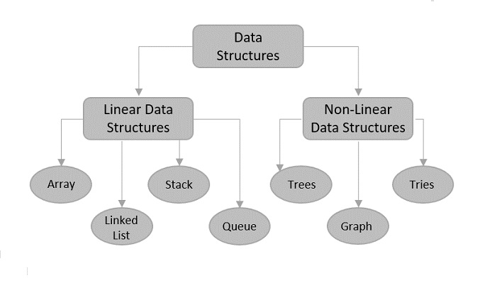
There are usually just two types of data structures −
Linear
Non-Linear
Linear Data Structures
The data is stored in linear data structures sequentially. These are rudimentary structures since the elements are stored one after the other without applying any mathematical operations.
Linear data structures are usually easy to implement but since the memory allocation might become complicated, time and space complexities increase. Few examples of linear data structures include −
Arrays
Linked Lists
Stacks
Queues
Based on the data storage methods, these linear data structures are divided into two sub-types. They are − static and dynamic data structures.
Static Linear Data Structures
In Static Linear Data Structures, the memory allocation is not scalable. Once the entire memory is used, no more space can be retrieved to store more data. Hence, the memory is required to be reserved based on the size of the program. This will also act as a drawback since reserving more memory than required can cause a wastage of memory blocks.
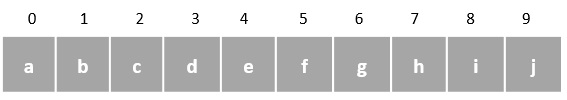
The best example for static linear data structures is an array.
Dynamic Linear Data Structures
In Dynamic linear data structures, the memory allocation can be done dynamically when required. These data structures are efficient considering the space complexity of the program.
Few examples of dynamic linear data structures include: linked lists, stacks and queues.
Non-Linear Data Structures
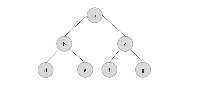
Non-Linear data structures store the data in the form of a hierarchy. Therefore, in contrast to the linear data structures, the data can be found in multiple levels and are difficult to traverse through.
However, they are designed to overcome the issues and limitations of linear data structures. For instance, the main disadvantage of linear data structures is the memory allocation. Since the data is allocated sequentially in linear data structures, each element in these data structures uses one whole memory block. However, if the data uses less memory than the assigned block can hold, the extra memory space in the block is wasted. Therefore, non-linear data structures are introduced. They decrease the space complexity and use the memory optimally.
This tutorial explains the basic terms related to data structure.
Data Definition
Data Definition defines a particular data with the following characteristics.
Atomic − Definition should define a single concept.
Traceable − Definition should be able to be mapped to some data element.
Accurate − Definition should be unambiguous.
Clear and Concise − Definition should be understandable.
Data Object
Data Object represents an object having a data.
Data Type
Data type is a way to classify various types of data such as integer, string, etc. which determines the values that can be used with the corresponding type of data, the type of operations that can be performed on the corresponding type of data. There are two data types −
Built-in Data Type
Derived Data Type
Built-in Data Type
Those data types for which a language has built-in support are known as Built-in Data types. For example, most of the languages provide the following built-in data types.
Integers
Boolean (true, false)
Floating (Decimal numbers)
Character and Strings
Derived Data Type
Those data types which are implementation independent as they can be implemented in one or the other way are known as derived data types. These data types are normally built by the combination of primary or built-in data types and associated operations on them. For example −
List
Array
Stack
Queue
Basic Operations
The data in the data structures are processed by certain operations. The particular data structure chosen largely depends on the frequency of the operation that needs to be performed on the data structure.
Asymptotic analysis of an algorithm refers to defining the mathematical foundation/framing of its run-time performance. Using asymptotic analysis, we can very well conclude the best case, average case, and worst case scenario of an algorithm.
Asymptotic analysis is input bound i.e., if there’s no input to the algorithm, it is concluded to work in a constant time. Other than the “input” all other factors are considered constant.
Asymptotic analysis refers to computing the running time of any operation in mathematical units of computation. For example, the running time of one operation is computed as f(n) and may be for another operation it is computed as g(n2). This means the first operation running time will increase linearly with the increase in n and the running time of the second operation will increase exponentially when n increases. Similarly, the running time of both operations will be nearly the same if n is significantly small.
Usually, the time required by an algorithm falls under three types −
Best Case − Minimum time required for program execution.
Average Case − Average time required for program execution.
Worst Case − Maximum time required for program execution.
Asymptotic Notations
Execution time of an algorithm depends on the instruction set, processor speed, disk I/O speed, etc. Hence, we estimate the efficiency of an algorithm asymptotically.
Time function of an algorithm is represented by T(n), where n is the input size.
Different types of asymptotic notations are used to represent the complexity of an algorithm. Following asymptotic notations are used to calculate the running time complexity of an algorithm.
O − Big Oh Notation
Ω − Big omega Notation
θ − Big theta Notation
o − Little Oh Notation
ω − Little omega Notation
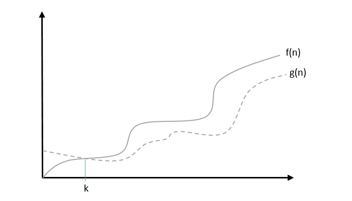
Big Oh, O: Asymptotic Upper Bound
The notation (n) is the formal way to express the upper bound of an algorithm’s running time. is the most commonly used notation. It measures the worst case time complexity or the longest amount of time an algorithm can possibly take to complete.
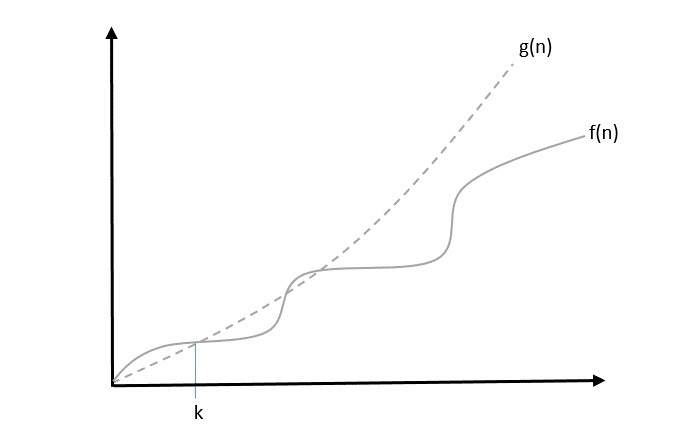
A function f(n) can be represented is the order of g(n) that is O(g(n)), if there exists a value of positive integer n as n0 and a positive constant c such that −
f(n)⩽c.g(n) for n>n0 in all case
Hence, function g(n) is an upper bound for function f(n), as g(n) grows faster than f(n).
Example
Let us consider a given function, f(n)=4.n3+10.n2+5.n+1
Considering g(n)=n3,
f(n)⩽5.g(n) for all the values of n>2
Hence, the complexity of f(n) can be represented as O(g(n)), i.e. O(n3)
Big Omega, Ω: Asymptotic Lower Bound
The notation Ω(n) is the formal way to express the lower bound of an algorithm’s running time. It measures the best case time complexity or the best amount of time an algorithm can possibly take to complete.
We say that f(n)=Ω(g(n)) when there exists constant c that f(n)⩾c.g(n) for all sufficiently large value of n. Here n is a positive integer. It means function g is a lower bound for function f ; after a certain value of n, f will never go below g.
Example
Let us consider a given function, f(n)=4.n3+10.n2+5.n+1.
Considering g(n)=n3, f(n)⩾4.g(n) for all the values of n>0.
Hence, the complexity of f(n) can be represented as Ω(g(n)), i.e. Ω(n3)
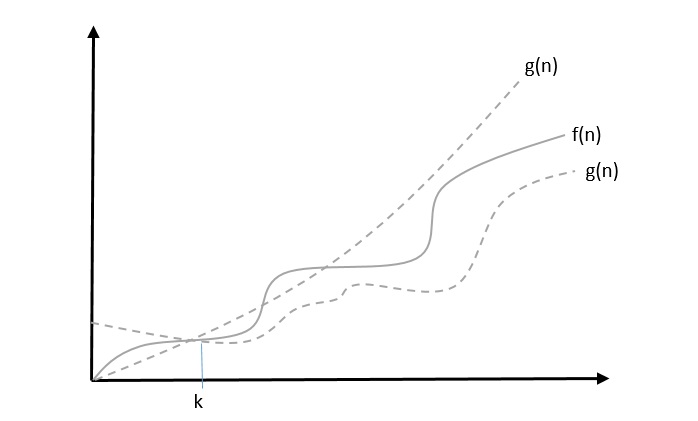
Theta, θ: Asymptotic Tight Bound
The notation (n) is the formal way to express both the lower bound and the upper bound of an algorithm’s running time. Some may confuse the theta notation as the average case time complexity; while big theta notation could be almost accurately used to describe the average case, other notations could be used as well.
We say that f(n)=θ(g(n)) when there exist constants c1 and c2 that c1.g(n)⩽f(n)⩽c2.g(n) for all sufficiently large value of n. Here n is a positive integer.
This means function g is a tight bound for function f.
Example
Let us consider a given function, f(n)=4.n3+10.n2+5.n+1
Considering g(n)=n3, 4.g(n)⩽f(n)⩽5.g(n) for all the large values of n.
Hence, the complexity of f(n) can be represented as θ(g(n)), i.e. θ(n3).
Little Oh, o
The asymptotic upper bound provided by O-notation may or may not be asymptotically tight. The bound 2.n2=O(n2) is asymptotically tight, but the bound 2.n=O(n2) is not.
We use o-notation to denote an upper bound that is not asymptotically tight.
We formally define o(g(n)) (little-oh of g of n) as the set f(n) = o(g(n)) for any positive constant c>0 and there exists a value n0>0, such that 0⩽f(n)⩽c.g(n).
Intuitively, in the o-notation, the function f(n) becomes insignificant relative to g(n) as n approaches infinity; that is,
limn→∞(f(n)g(n))=0
Example
Let us consider the same function, f(n)=4.n3+10.n2+5.n+1
Considering g(n)=n4,
limn→∞(4.n3+10.n2+5.n+1n4)=0
Hence, the complexity of f(n) can be represented as o(g(n)), i.e. o(n4).
Little Omega, ω
We use ω-notation to denote a lower bound that is not asymptotically tight. Formally, however, we define ω(g(n)) (little-omega of g of n) as the set f(n) = ω(g(n)) for any positive constant C > 0 and there exists a value n0>0, such that $0 \leqslant c.g(n)
For example, n22=ω(n), but n22≠ω(n2). The relation f(n)=ω(g(n)) implies that the following limit exists
limn→∞(f(n)g(n))=∞
That is, f(n) becomes arbitrarily large relative to g(n) as n approaches infinity.
Example
Let us consider same function, f(n)=4.n3+10.n2+5.n+1
Considering g(n)=n2,
limn→∞(4.n3+10.n2+5.n+1n2)=∞
Hence, the complexity of f(n) can be represented as o(g(n)), i.e. ω(n2).
Common Asymptotic Notations
Following is a list of some common asymptotic notations −
constant
−
O(1)
logarithmic
−
O(log n)
linear
−
O(n)
n log n
−
O(n log n)
quadratic
−
O(n2)
cubic
−
O(n3)
polynomial
−
nO(1)
exponential
−
2O(n)
Apriori and Apostiari Analysis
Apriori analysis means, analysis is performed prior to running it on a specific system. This analysis is a stage where a function is defined using some theoretical model. Hence, we determine the time and space complexity of an algorithm by just looking at the algorithm rather than running it on a particular system with a different memory, processor, and compiler.
Apostiari analysis of an algorithm means we perform analysis of an algorithm only after running it on a system. It directly depends on the system and changes from system to system.
In an industry, we cannot perform Apostiari analysis as the software is generally made for an anonymous user, which runs it on a system different from those present in the industry.
In Apriori, it is the reason that we use asymptotic notations to determine time and space complexity as they change from computer to computer; however, asymptotically they are the same.
Algorithm is a step-by-step procedure, which defines a set of instructions to be executed in a certain order to get the desired output. Algorithms are generally created independent of underlying languages, i.e. an algorithm can be implemented in more than one programming language.
From the data structure point of view, following are some important categories of algorithms −
Search − Algorithm to search an item in a data structure.
Sort − Algorithm to sort items in a certain order.
Insert − Algorithm to insert item in a data structure.
Update − Algorithm to update an existing item in a data structure.
Delete − Algorithm to delete an existing item from a data structure.
Characteristics of an Algorithm
Not all procedures can be called an algorithm. An algorithm should have the following characteristics −
Unambiguous − Algorithm should be clear and unambiguous. Each of its steps (or phases), and their inputs/outputs should be clear and must lead to only one meaning.
Input − An algorithm should have 0 or more well-defined inputs.
Output − An algorithm should have 1 or more well-defined outputs, and should match the desired output.
Finiteness − Algorithms must terminate after a finite number of steps.
Feasibility − Should be feasible with the available resources.
Independent − An algorithm should have step-by-step directions, which should be independent of any programming code.
How to Write an Algorithm?
There are no well-defined standards for writing algorithms. Rather, it is problem and resource dependent. Algorithms are never written to support a particular programming code.
As we know that all programming languages share basic code constructs like loops (do, for, while), flow-control (if-else), etc. These common constructs can be used to write an algorithm.
We write algorithms in a step-by-step manner, but it is not always the case. Algorithm writing is a process and is executed after the problem domain is well-defined. That is, we should know the problem domain, for which we are designing a solution.
Example
Let’s try to learn algorithm-writing by using an example.
Problem − Design an algorithm to add two numbers and display the result.
Step 1 − START
Step 2 − declare three integers a, b & cStep 3 − define values of a & bStep 4 − add values of a & bStep 5 − store output of step 4 to cStep 6 − print cStep 7 − STOP
Algorithms tell the programmers how to code the program. Alternatively, the algorithm can be written as −
Step 1 − START ADD
Step 2 − get values of a & bStep 3 − c ← a + b
Step 4 − display c
Step 5 − STOP
In design and analysis of algorithms, usually the second method is used to describe an algorithm. It makes it easy for the analyst to analyze the algorithm ignoring all unwanted definitions. He can observe what operations are being used and how the process is flowing.
Writing step numbers, is optional.
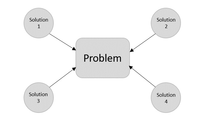
We design an algorithm to get a solution of a given problem. A problem can be solved in more than one ways.
Hence, many solution algorithms can be derived for a given problem. The next step is to analyze those proposed solution algorithms and implement the best suitable solution.
Algorithm Analysis
Efficiency of an algorithm can be analyzed at two different stages, before implementation and after implementation. They are the following −
A Priori Analysis − This is a theoretical analysis of an algorithm. Efficiency of an algorithm is measured by assuming that all other factors, for example, processor speed, are constant and have no effect on the implementation.
A Posterior Analysis − This is an empirical analysis of an algorithm. The selected algorithm is implemented using programming language. This is then executed on target computer machine. In this analysis, actual statistics like running time and space required, are collected.
We shall learn about a priori algorithm analysis. Algorithm analysis deals with the execution or running time of various operations involved. The running time of an operation can be defined as the number of computer instructions executed per operation.
Algorithm Complexity
Suppose X is an algorithm and n is the size of input data, the time and space used by the algorithm X are the two main factors, which decide the efficiency of X.
Time Factor − Time is measured by counting the number of key operations such as comparisons in the sorting algorithm.
Space Factor − Space is measured by counting the maximum memory space required by the algorithm.
The complexity of an algorithm f(n) gives the running time and/or the storage space required by the algorithm in terms of n as the size of input data.
Space Complexity
Space complexity of an algorithm represents the amount of memory space required by the algorithm in its life cycle. The space required by an algorithm is equal to the sum of the following two components −
A fixed part that is a space required to store certain data and variables, that are independent of the size of the problem. For example, simple variables and constants used, program size, etc.
A variable part is a space required by variables, whose size depends on the size of the problem. For example, dynamic memory allocation, recursion stack space, etc.
Space complexity S(P) of any algorithm P is S(P) = C + SP(I), where C is the fixed part and S(I) is the variable part of the algorithm, which depends on instance characteristic I. Following is a simple example that tries to explain the concept −
Algorithm: SUM(A, B)
Step 1 − START
Step 2 − C ← A + B + 10
Step 3 − Stop
Here we have three variables A, B, and C and one constant. Hence S(P) = 1 + 3. Now, space depends on data types of given variables and constant types and it will be multiplied accordingly.
Time Complexity
Time complexity of an algorithm represents the amount of time required by the algorithm to run to completion. Time requirements can be defined as a numerical function T(n), where T(n) can be measured as the number of steps, provided each step consumes constant time.
For example, addition of two n-bit integers takes n steps. Consequently, the total computational time is T(n) = c ∗ n, where c is the time taken for the addition of two bits. Here, we observe that T(n) grows linearly as the input size increases.
If you are still willing to set up your own environment for C programming language, you need the following two tools available on your computer, (a) Text Editor and (b) The C Compiler.
Text Editor
This will be used to type your program. Examples of few editors include Windows Notepad, OS Edit command, Brief, Epsilon, EMACS, and vim or vi.
The name and the version of the text editor can vary on different operating systems. For example, Notepad will be used on Windows, and vim or vi can be used on Windows as well as Linux or UNIX.
The files you create with your editor are called source files and contain program source code. The source files for C programs are typically named with the extension “.c“.
Before starting your programming, make sure you have one text editor in place and you have enough experience to write a computer program, save it in a file, compile it, and finally execute it.
The C Compiler
The source code written in the source file is the human readable source for your program. It needs to be “compiled”, to turn into machine language so that your CPU can actually execute the program as per the given instructions.
This C programming language compiler will be used to compile your source code into a final executable program. We assume you have the basic knowledge about a programming language compiler.
Most frequently used and free available compiler is GNU C/C++ compiler. Otherwise, you can have compilers either from HP or Solaris if you have respective Operating Systems (OS).
The following section guides you on how to install GNU C/C++ compiler on various OS. We are mentioning C/C++ together because GNU GCC compiler works for both C and C++ programming languages.
Installation on UNIX/Linux
If you are using Linux or UNIX, then check whether GCC is installed on your system by entering the following command from the command line −
$ gcc -v
If you have GNU compiler installed on your machine, then it should print a message such as the following −
Using built-in specs.
Target: i386-redhat-linux
Configured with: ../configure --prefix = /usr .......
Thread model: posix
gcc version 4.1.2 20080704 (Red Hat 4.1.2-46)
If GCC is not installed, then you will have to install it yourself using the detailed instructions available at https://gcc.gnu.org/install/
This tutorial has been written based on Linux and all the given examples have been compiled on Cent OS flavor of Linux system.
Installation on Mac OS
If you use Mac OS X, the easiest way to obtain GCC is to download the Xcode development environment from Apple’s website and follow the simple installation instructions. Once you have Xcode setup, you will be able to use GNU compiler for C/C++.
To install GCC on Windows, you need to install MinGW. To install MinGW, go to the MinGW homepage, www.mingw.org, and follow the link to the MinGW download page. Download the latest version of the MinGW installation program, which should be named MinGW-<version>.exe.
While installing MinWG, at a minimum, you must install gcc-core, gcc-g++, binutils, and the MinGW runtime, but you may wish to install more.
Add the bin subdirectory of your MinGW installation to your PATH environment variable, so that you can specify these tools on the command line by their simple names.
When the installation is complete, you will be able to run gcc, g++, ar, ranlib, dlltool, and several other GNU tools from the Windows command line.
Data Structure is a systematic way to organize data in order to use it efficiently. Following terms are the foundation terms of a data structure.
Interface − Each data structure has an interface. Interface represents the set of operations that a data structure supports. An interface only provides the list of supported operations, type of parameters they can accept and return type of these operations.
Implementation − Implementation provides the internal representation of a data structure. Implementation also provides the definition of the algorithms used in the operations of the data structure.
Types of Data Structures
Here are different type of data structures which we are going to learn in this tutorial:
Algorithm is a step-by-step procedure, which defines a set of instructions to be executed in a certain order to get the desired output. Algorithms are generally created independent of underlying languages, i.e. an algorithm can be implemented in more than one programming language.
Types of Algorithms
Here are different type of algorithms which we are going to learn in this tutorial:
Correctness − Data structure implementation should implement its interface correctly.
Time Complexity − Running time or the execution time of operations of data structure must be as small as possible.
Space Complexity − Memory usage of a data structure operation should be as little as possible.
Execution Time Cases
There are three cases which are usually used to compare various data structure’s execution time in a relative manner.
Worst Case − This is the scenario where a particular data structure operation takes maximum time it can take. If an operation’s worst case time is ƒ(n) then this operation will not take more than ƒ(n) time where ƒ(n) represents function of n.
Average Case − This is the scenario depicting the average execution time of an operation of a data structure. If an operation takes ƒ(n) time in execution, then m operations will take mƒ(n) time.
Best Case − This is the scenario depicting the least possible execution time of an operation of a data structure. If an operation takes ƒ(n) time in execution, then the actual operation may take time as the random number which would be maximum as ƒ(n).
Basic DSA Terminologies
Data − Data are values or set of values.
Data Item − Data item refers to single unit of values.
Group Items − Data items that are divided into sub items are called as Group Items.
Elementary Items − Data items that cannot be divided are called as Elementary Items.
Attribute and Entity − An entity is that which contains certain attributes or properties, which may be assigned values.
Entity Set − Entities of similar attributes form an entity set.
Field − Field is a single elementary unit of information representing an attribute of an entity.
Record − Record is a collection of field values of a given entity.
File − File is a collection of records of the entities in a given entity set.
Data structures and algorithms (DSA) are two important aspects of any programming language. Every programming language has its own data structures and different types of algorithms to handle these data structures.
Data Structures are used to organise and store data to use it in an effective way when performing data operations.
Algorithm is a step-by-step procedure, which defines a set of instructions to be executed in a certain order to get the desired output. Algorithms are generally created independent of underlying languages, i.e. an algorithm can be implemented in more than one programming language.
Almost every enterprise application uses various types of data structures in one or the other way. So, as a programmer, data structures and algorithms are really important aspects of day-to-day programming.
A data structure is a particular way to arrange data so it can be saved in memory and retrieved for later use where as an algorithm is a set of steps for solving a known problem. Data Structures and Algorithms is abbreviated as DSA in the context of Computer Science.
This tutorial will give you a great understanding on Data Structures needed to understand the complexity of enterprise level applications and need of algorithms, and data structures.
Why to Learn Data Structures & Algorithms (DSA)?
As applications are getting complex and data rich, there are three common problems that applications face now-a-days.
Data Search − Consider an inventory of 1 million(106) items of a store. If the application is to search an item, it has to search an item in 1 million(106) items every time slowing down the search. As data grows, search will become slower.
Processor speed − Processor speed although being very high, falls limited if the data grows to billion records.
Multiple requests − As thousands of users can search data simultaneously on a web server, even the fast server fails while searching the data.
To solve the above-mentioned problems, data structures come to rescue. Data can be organized in a data structure in such a way that all items may not be required to be searched, and the required data can be searched almost instantly.
How to start learning Data Structures & Algorithms (DSA)?
The basic steps to learn DSA is as follows:
Step 1 – Learn Time and Space complexities
Time and Space complexities are the measures of the amount of time required to execute the code (Time Complexity) and amount of space required to execute the code (Space Complexity).
Step 2 – Learn Different Data Structures
Here we learn different types of data structures like Array, Stack, Queye, Linked List et.
Step 3 – Learn Different Algorithms
Once you have good undertanding about various data sturtcures then you can start learning associated algorithms to process the data stored in these data structures. These algorithms include searching, sorting, and other different algorithms.
Applications of Data Structures & Algorithms (DSA)
From the data structure point of view, following are some important categories of algorithms −
Search − Algorithm to search an item in a data structure.
Sort − Algorithm to sort items in a certain order.
Insert − Algorithm to insert item in a data structure.
Update − Algorithm to update an existing item in a data structure.
Delete − Algorithm to delete an existing item from a data structure.
The following computer problems can be solved using Data Structures −
Fibonacci number series
Knapsack problem
Tower of Hanoi
All pair shortest path by Floyd-Warshall
Shortest path by Dijkstra
Project scheduling
Who Should Learn DSA
This tutorial has been designed for Computer Science Students as well as Software Professionals who are willing to learn data Structures and Algorithm (DSA) Programming in simple and easy steps.
After completing this tutorial you will be at intermediate level of expertise from where you can take yourself to higher level of expertise.
DSA Online Editor & Compiler
In this tutorial, we will work with data structures and algorithms in four different programming languages: C, C++, Java, Python. So, we provide Online Compilers for each of these languages to execute the given code. Doing so, we are aiming to compromise the need for local setup for the compilers.
#include <stdio.h>intmain(){int LA[3]={}, i;for(i =0; i <3; i++){
      LA[i]= i +2;printf("LA[%d] = %d \n", i, LA[i]);}return0;}
Output
LA [0] = 2
LA [1] = 3
LA [2] = 4
Prerequisites to Learn DSA
Before proceeding with this tutorial, you should have a basic understanding of C programming language, text editor, and execution of programs, etc.
DSA Jobs and Opportunities
Professionals in DSA are in high demands as more and more organizations rely on them to solve complex problems and make data-driven decisions. You can earn competitive salaries, and the specific pay can vary based on your location, experience, and job role.
Many top companies are actively recruiting experts in DSA, and they offer roles such as Software Engineer, Data Scientist, Machine Learning Engineer, and more. These companies need individuals who can solve complex problems, analyse data, and create algorithms to drive their business forward. Here is the list of few such companies −
Google
Amazon
Microsoft
Apple
Adobe
JPMorgan Chase
Goldman Sachs
Walmart
Johnson & Johnson
Airbnb
Tesla
These are just a few examples, and the demand for DSA professionals is continually growing across various sectors. By developing expertise in these areas, you can open up a wide range of career opportunities in some of the world’s leading companies.
To get started, there are user-friendly tutorials and resources available to help you master DSA. These materials are designed to prepare you for technical interviews and certification exams, and you can learn at your own pace, anytime and anywhere.
Frequently Asked Questions about DSA
There are many Frequently Asked Questions (FAQs) on Data Structures and Algorithms due to the complex nature of this concept. In this section, we will try to answer some of them briefly.
1:What Are Data Structures and Algorithms?
A data structure is a collection of similar or different data types, and is used to store and modify data using programming languages. And, an algorithm is defined as a set of instructions that must be followed to solve a problem.
Data Structures and Algorithms is a study of such data structures and the algorithms that use them.
2:What is the best programming language for data structures and algorithms?
The best programming language to work with data structures is C++, due to its efficiency and abundant resources for data structures. Despite that, any programming language can be the best pick to work with data structures if you are fluent in it.
3:Which is the best place to learn Data Structures?
Here are the summarized list of tips which you can follow to start learning Data Structures.
Follow our tutorial step by step from the very beginning.
Read more articles, watch online courses or buy reference books on Data Structures to enhance your knowledge.
Try to execute a small program using data structures in any programming language to check your knowledge in these concepts.
4:Is array a Data Type or Data Structure?
A datatype is a type of value a variable holds. These values can be numeric, string, characters, etc. An array is defined as a collection of similar type of values stored together. Hence, it is more likely to be a data structures storing values of same datatype.
5:What Should I Learn First: Data Structures or Algorithms?
Data Structures organize the data used in algorithms. They are the foundation of computations performed using algorithms. Hence, learning data structures is recommended first, as it becomes easier to understand the concept of Algorithms with all the prior knowledge.
6:Data Structures and Algorithms in Real Life!
Not only in software development, but we can observe the use of data structures in our day-to-day life as well. For instance, piling up plates and removing them one-by-one is the simpler example on how stack data structure organizes its data. Similarly, queueing up to buy movie tickets has the same mechanism as inserting and deleting the data from a queue.
In software development, developing navigation maps using graph data structure is also a common real life application.
7:Need of Data Structures and Algorithms for Deep Learning and Machine Learning?
Machine Learning and Deep Learning work with mathematical computations and large sets of data. Organizing this data properly becomes crucial in order to process these data-sets for training and deploying suitable models on them. Hence, having a deep knowledge in Data Structures and Algorithms is important while working with Machine Learning and Deep Learning.
8:What is The Difference Between Data Type and Data Structure?
A datatype defines the type of value stored in a variable. This decides the type of operations performed and functions called on these values. Whereas, a data structure is a collection of similar or different types of data, which is used to organize and manipulate data in a program.
PHP is very rich in terms of Built-in functions. Here is the list of various important function categories. There are various other function categories which are not covered here.
Select a category to see a list of all the functions related to that category.
PDO is an acronym for PHP Data Objects. PHP can interact with most of the relational as well as NOSQL databases. The default PHP installation comes with vendor-specific database extensions already installed and enabled. In addition to such database drivers specific to a certain type of database, such as the mysqli extension for MySQL, PHP also supports abstraction layers such as PDO and ODBC.
The PDO extension defines a lightweight, consistent interface for accessing databases in PHP. The functionality of each vendor-specific extension varies from the other. As a result, if you intend to change the backend database of a certain PHP application, say from PostGreSql to MySQL, you need to make a lot of changes to the code. The PDO API on the other hand doesnt require any changes apart from specifying the URL and the credentials of the new database to be used.
Your current PHP installation must have the corresponding PDO driver available to be able to work with. Currently the following databases are supported with the corresponding PDO interfaces −
Driver Name
Supported Databases
PDO_CUBRID
Cubrid
PDO_DBLIB
FreeTDS / Microsoft SQL Server / Sybase
PDO_FIREBIRD
Firebird
PDO_IBM
IBM DB2
PDO_INFORMIX
IBM Informix Dynamic Server
PDO_MYSQL
MySQL 3.x/4.x/5.x/8.x
PDO_OCI
Oracle Call Interface
PDO_ODBC
ODBC v3 (IBM DB2, unixODBC and win32 ODBC)
PDO_PGSQL
PostgreSQL
PDO_SQLITE
SQLite 3 and SQLite 2
PDO_SQLSRV
Microsoft SQL Server / SQL Azure
By default, the PDO_SQLITE driver is enabled in the settings of php.ini, so if you wish to interact with a MySQL database with PDO, make sure that the following line is uncommented by removing the leading semicolon.
extension=pdo_mysql
You can obtain the list of currently available PDO drivers by calling PDO::getAvailableDrivers() static function in PDO class.
PDO Connection
An instance of PDO base class represents a database connection. The constructor accepts parameters for specifying the database source (known as the DSN) and optionally for the username and password (if any).
The following snippet is a typical way of establishing connection with a MySQL database −
<?php
   $dbh = new PDO('mysql:host=localhost;dbname=test', $user, $pass);
?>
If there is any connection error, a PDOException object will be thrown.
The PDO class defines the following static methods −
PDO::beginTransaction
After obtaining the connection object, you should call this method to that initiates a transaction.
publicPDO::beginTransaction():bool
This method turns off autocommit mode. Hence, you need to call commit() method to make persistent changes to the database Calling rollBack() will roll back all changes to the database and return the connection to autocommit mode.This method returns true on success or false on failure.
PDO::commit
The commit() method commits a transaction.
publicPDO::commit():bool
Since the BeginTransaction disables the autocommit mode, you should call this method after a transaction. It commits a transaction, returning the database connection to autocommit mode until the next call to PDO::beginTransaction() starts a new transaction. This method returns true on success or false on failure.
PDO::exec
The exec() method executes an SQL statement and return the number of affected rows
publicPDO::exec(string$statement):int|false
The exec() method executes an SQL statement in a single function call, returning the number of rows affected by the statement.
Note that it does not return results from a SELECT statement. If you have a SELECT statement that is to be executed only once during your program, consider issuing PDO::query().
On the other hand For a statement that you need to issue multiple times, prepare a PDOStatement object with PDO::prepare() and issue the statement with PDOStatement::execute().
The exec() method need a string parameter that represents a SQL statement to prepare and execute, and returns the number of rows that were modified or deleted by the SQL statement you issued. If no rows were affected, PDO::exec() returns 0.
PDO::query
The query() method prepares and executes an SQL statement without placeholders
This method prepares and executes an SQL statement in a single function call, returning the statement as a PDOStatement object.
PDO::rollBack
The rollback() method rolls back a transaction as initiated by PDO::beginTransaction().
publicPDO::rollBack():bool
If the database was set to autocommit mode, this function will restore autocommit mode after it has rolled back the transaction.
Note that some databases, including MySQL, automatically issue an implicit COMMIT when a DDL statement such as DROP TABLE or CREATE TABLE is issued within a transaction, and hence it will prevent you from rolling back any other changes within the transaction boundary. This method returns true on success or false on failure.
Example
The following code creates a student table in the myDB database on a MySQL server.
<?php
   $dsn="localhost";
   $dbName="myDB";
   $username="root";
   $password="";
   try{
      $conn= new PDO("mysql:host=$dsn;dbname=$dbName",$username,$password);
      Echo "Successfully connected with $dbName database";
      $qry = <<<STRING
      CREATE TABLE IF NOT EXISTS STUDENT (
         student_id INT AUTO_INCREMENT,
         name VARCHAR(255) NOT NULL,
         marks INTEGER(3),
         PRIMARY KEY (student_id)
      );
      STRING;
      echo $qry . PHP_EOL;
      $conn->exec($qry);
      $conn->commit();
      echo "Table created\n";
   }
   catch(Exception $e){
      echo "Connection failed : " . $e->getMessage();
   }
?>
Example
Use the following code to insert a new record in student table created in the above example −
<?php
   $dsn="localhost";
   $dbName="myDB";
   $username="root";
   $password="";
   try {
      $conn= new PDO("mysql:host=$dsn;dbname=$dbName",$username,$password);
      echo "Successfully connected with $dbName database";

      $sql = "INSERT INTO STUDENT values(1, 'Raju', 60)";
      $conn->exec($sql);
      $conn->commit();
      echo "A record inserted\n";
   } catch(Exception $e){
      echo "Connection failed : " . $e->getMessage();
   }
?>
Example
The following PHP script fetches all the records in the student table −
PHP FastCGI Process Manager (PHP-FPM) is an efficient alternative to traditional CGI-based methods for handling PHP requests, particularly in high-traffic environments. PHP-FPM has a number of important features. These features are as follows −
Reduced Memory Consumption
With the help of a pool of worker processes to handle requests PHP-FPM significantly reduces memory overhead compared to traditional CGI methods that spawn a new process for each request.
Improved Performance
PHP-FPM’s worker processes are persistent. It allows them to handle multiple requests. It doesnt need ti repeatedly create and destroy processes. This leads to faster response times and improved handling of high concurrency.
Enhanced Scalability
PHP-FPM’s pool of worker processes can be dynamically adjusted based on traffic demands, allowing it to scale effectively to handle varying workloads.
Advanced Process Management
PHP-FPM offers graceful startup and shutdown. It also has granular control over process management, including, emergency restarts, and monitoring of worker processes.
Environment Isolation
PHP-FPM enables the creation of separate pools for different applications or user groups, so that better isolation and security can be provided for each environment.
Customizable Configuration
PHP-FPM uses php.ini based configuration options. With these extensive options, fine-tuning of its behavior is possible to match specific application requirements.
Supports multiple PHP Versions
PHP-FPM can manage multiple PHP versions simultaneously, enabling the deployment of different PHP applications on a single server.
PHP-FPM is commonly used with web servers like Nginx or Apache. It acts as a backend processor for handling PHP requests. It has become the preferred method for managing PHP applications in production environments due to its performance, scalability, and reliability.