Graph Data Structure

What is a Graph?

A graph is an abstract data type (ADT) which consists of a set of objects that are connected to each other via links. The interconnected objects are represented by points termed as vertices, and the links that connect the vertices are called edges.

Formally, a graph is a pair of sets (V, E), where V is the set of vertices and E is the set of edges, connecting the pairs of vertices. Take a look at the following graph −

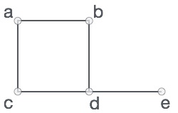
In the above graph,

V = {a, b, c, d, e}

E = {ab, ac, bd, cd, de}

Graph Data Structure

Mathematical graphs can be represented in data structure. We can represent a graph using an array of vertices and a two-dimensional array of edges. Before we proceed further, let’s familiarize ourselves with some important terms −

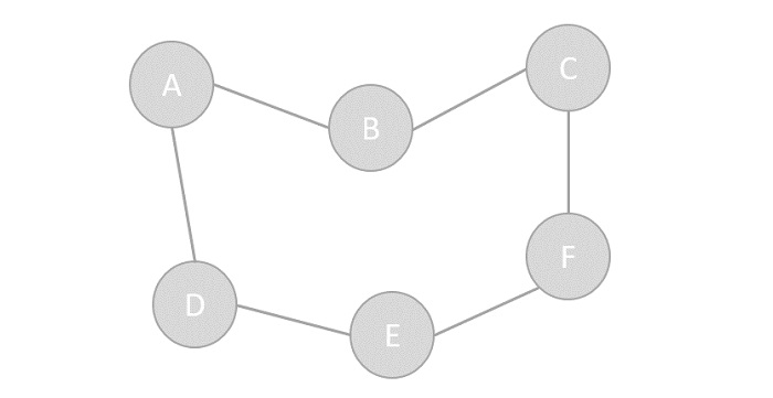
• Vertex − Each node of the graph is represented as a vertex. In the following example, the labeled circle represents vertices. Thus, A to G are vertices. We can represent them using an array as shown in the following image. Here A can be identified by index 0. B can be identified using index 1 and so on.
• Edge − Edge represents a path between two vertices or a line between two vertices. In the following example, the lines from A to B, B to C, and so on represents edges. We can use a two-dimensional array to represent an array as shown in the following image. Here AB can be represented as 1 at row 0, column 1, BC as 1 at row 1, column 2 and so on, keeping other combinations as 0.
• Adjacency − Two node or vertices are adjacent if they are connected to each other through an edge. In the following example, B is adjacent to A, C is adjacent to B, and so on.
• Path − Path represents a sequence of edges between the two vertices. In the following example, ABCD represents a path from A to D.

Operations of Graphs

The primary operations of a graph include creating a graph with vertices and edges, and displaying the said graph. However, one of the most common and popular operation performed using graphs are Traversal, i.e. visiting every vertex of the graph in a specific order.

There are two types of traversals in Graphs −

• Depth First Search Traversal
• Breadth First Search Traversal

Depth First Search Traversal

Depth First Search is a traversal algorithm that visits all the vertices of a graph in the decreasing order of its depth. In this algorithm, an arbitrary node is chosen as the starting point and the graph is traversed back and forth by marking unvisited adjacent nodes until all the vertices are marked.

The DFS traversal uses the stack data structure to keep track of the unvisited nodes.

Click and check Depth First Search Traversal

Breadth First Search Traversal

Breadth First Search is a traversal algorithm that visits all the vertices of a graph present at one level of the depth before moving to the next level of depth. In this algorithm, an arbitrary node is chosen as the starting point and the graph is traversed by visiting the adjacent vertices on the same depth level and marking them until there is no vertex left.

The DFS traversal uses the queue data structure to keep track of the unvisited nodes.

Click and check Breadth First Search Traversal

Representation of Graphs

While representing graphs, we must carefully depict the elements (vertices and edges) present in the graph and the relationship between them. Pictorially, a graph is represented with a finite set of nodes and connecting links between them. However, we can also represent the graph in other most commonly used ways, like −

• Adjacency Matrix
• Adjacency List

Adjacency Matrix

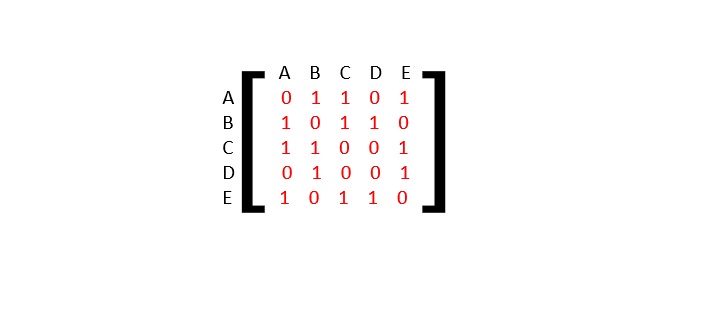
The Adjacency Matrix is a V x V matrix where the values are filled with either 0 or 1. If the link exists between Vi and Vj, it is recorded 1; otherwise, 0.

For the given graph below, let us construct an adjacency matrix −

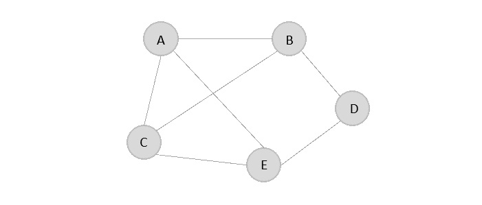
The adjacency matrix is −

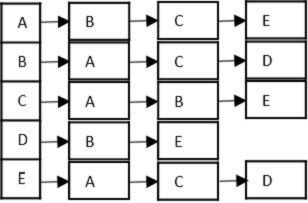
Adjacency List

The adjacency list is a list of the vertices directly connected to the other vertices in the graph.

The adjacency list is −

Types of graph

There are two basic types of graph −

• Directed Graph
• Undirected Graph

Directed graph, as the name suggests, consists of edges that possess a direction that goes either away from a vertex or towards the vertex. Undirected graphs have edges that are not directed at all.

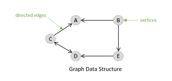
Directed Graph

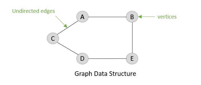
Undirected Graph

Spanning Tree

A spanning tree is a subset of an undirected graph that contains all the vertices of the graph connected with the minimum number of edges in the graph. Precisely, the edges of the spanning tree is a subset of the edges in the original graph.

If all the vertices are connected in a graph, then there exists at least one spanning tree. In a graph, there may exist more than one spanning tree.

Properties

• A spanning tree does not have any cycle.
• Any vertex can be reached from any other vertex.

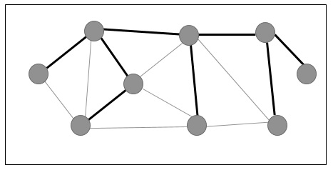
Example

In the following graph, the highlighted edges form a spanning tree.

Minimum Spanning Tree

A Minimum Spanning Tree (MST) is a subset of edges of a connected weighted undirected graph that connects all the vertices together with the minimum possible total edge weight. To derive an MST, Prim’s algorithm or Kruskal’s algorithm can be used. Hence, we will discuss Prim’s algorithm in this chapter.

As we have discussed, one graph may have more than one spanning tree. If there are n number of vertices, the spanning tree should have n − l1 number of edges. In this context, if each edge of the graph is associated with a weight and there exists more than one spanning tree, we need to find the minimum spanning tree of the graph.

Moreover, if there exist any duplicate weighted edges, the graph may have multiple minimum spanning tree.

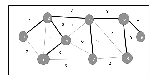
In the above graph, we have shown a spanning tree though it’s not the minimum spanning tree. The cost of this spanning tree is (5+7+3+3+5+8+3+4)=38.

Shortest Path

The shortest path in a graph is defined as the minimum cost route from one vertex to another. This is most commonly seen in weighted directed graphs but are also applicable to undirected graphs.

A popular real−world application of finding the shortest path in a graph is a map. Navigation is made easier and simpler with the various shortest path algorithms where destinations are considered vertices of the graph and routes are the edges. The two common shortest path algorithms are −

• Dijkstra’s Shortest Path Algorithm
• Bellman Ford’s Shortest Path Algorithm

Example

Following are the implementations of this operation in various programming languages −

CC++JavaPython

#include <stdio.h>#include <stdlib.h>#include <stdlib.h>#define V 5 // Maximum number of vertices in the graphstructgraph{// declaring graph data structurestructvertex*point[V];};structvertex{// declaring verticesint end;structvertex*next;};structEdge{// declaring edgesint end, start;};structgraph*create_graph(structEdge edges[],int x){int i;structgraph*graph =(structgraph*)malloc(sizeof(structgraph));for(i =0; i < V; i++){
      graph->point[i]=NULL;}for(i =0; i < x; i++){int start = edges[i].start;int end = edges[i].end;structvertex*v =(structvertex*)malloc(sizeof(structvertex));
      v->end = end;
      v->next = graph->point[start];
      graph->point[start]= v;}return graph;}intmain(){structEdge edges[]={{0,1},{0,2},{0,3},{1,2},{1,4},{2,4},{2,3},{3,1}};int n =sizeof(edges)/sizeof(edges[0]);structgraph*graph =create_graph(edges, n);printf("The graph created is: ");for(int i =0; i < V; i++){structvertex*ptr = graph->point[i];while(ptr !=NULL){printf("(%d -> %d)\t", i, ptr->end);
         ptr = ptr->next;}printf("\n");}return0;}

Output

The graph created is:
(1 -> 3)	(1 -> 0)	
(2 -> 1)	(2 -> 0)	
(3 -> 2)	(3 -> 0)	
(4 -> 2)	(4 -> 1)