Category: Randomized Algorithms

  • Fisher-Yates Shuffle Algorithm

    The Fisher-Yates Shuffle algorithm shuffles a finite sequence of elements by generating a random permutation. The possibility of every permutation occurring is equally likely. The algorithm is performed by storing the elements of the sequence in a sack and drawing each element randomly from the sack to form the shuffled sequence.

    Coined after Ronald Fisher and Frank Yates, for designing the original method of the shuffle, the algorithm is unbiased. It generates all permutations in same conditions so the output achieved is nowhere influenced. However, the modern version of the Fisher-Yates Algorithm is more efficient than that of the original one.

    Fisher-Yates Algorithm

    The Original Method

    The original method of Shuffle algorithm involved a pen and paper to generate a random permutation of a finite sequence. The algorithm to generate the random permutation is as follows −

    Step 1 − Write down all the elements in the finite sequence. Declare a separate list to store the output achieved.

    Step 2 − Choose an element i randomly in the input sequence and add it onto the output list. Mark the element i as visited.

    Step 3 − Repeat Step 2 until all the element in the finite sequence is visited and added onto the output list randomly.

    Step 4 − The output list generated after the process terminates is the random permutation generated.

    The Modern Algorithm

    The modern algorithm is a slightly modified version of the original fisher-yates shuffle algorithm. The main goal of the modification is to computerize the original algorithm by reducing the time complexity of the original method. The modern method is developed by Richard Durstenfeld and was popularized by Donald E. Knuth.

    Therefore, the modern method makes use of swapping instead of maintaining another output list to store the random permutation generated. The time complexity is reduced to O(n) rather than O(n2). The algorithm goes as follows −

    Step 1 − Write down the elements 1 to n in the finite sequence.

    Step 2 − Choose an element i randomly in the input sequence and swap it with the last unvisited element in the list.

    Step 3 − Repeat Step 2 until all the element in the finite sequence is visited and swapped.

    Step 4 − The list generated after the process terminates is the random permutation sequence.

    Pseudocode

    Shuffling is done from highest index to the lowest index of the array in the following modern method pseudocode.

    Fisher-Yates Shuffle (array of n elements):
    for i from n1 downto 1 do
       j ← random integer such that 0  j  i
       exchange a[j] and a[i]
    

    Shuffling is done from lowest index to the highest index of the array in the following modern method pseudocode.

    Fisher-Yates Shuffle (array of n elements):
    for i from 0 to n2 do
       j ← random integer such that i  j < n
       exchange a[i] and a[j]
    

    Original Method Example

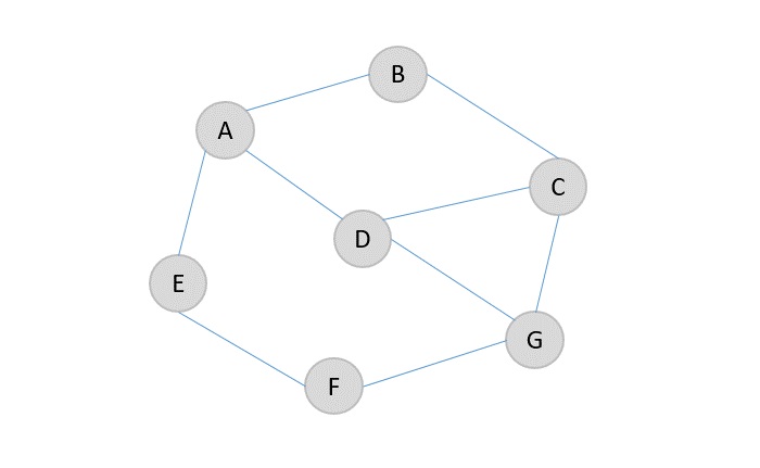
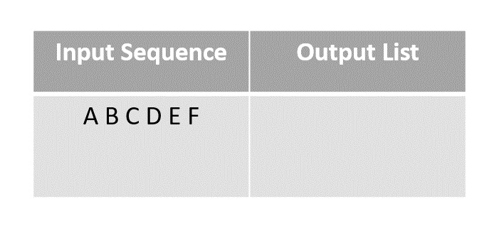
    To describe the algorithm better, let us permute the the given finite sequence of the first six letters of the alphabet. Input sequence: A B C D E F.

    Step 1

    This is called the pen and paper method. We consider an input array with the finite sequence stored and an output array to store the result.
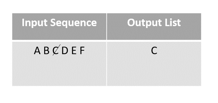
    input_sequence

    Step 2

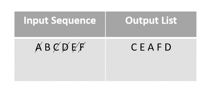
    Choose any element randomly and add it onto the output list after marking it checked. In this case, we choose element C.
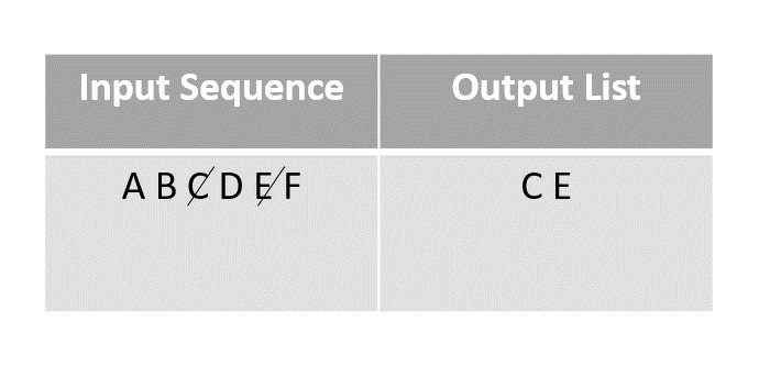
    output_list

    Step 3

    The next element chosen randomly is E which is marked and added to the output list.
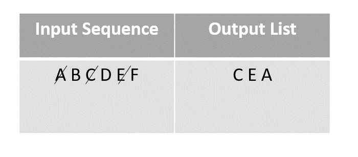
    chosen_randomly_E

    Step 4

    The random function then picks the next element A and adds it onto the output array after marking it visited.
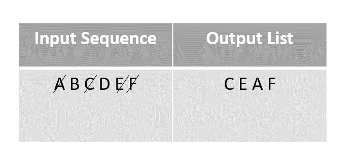
    next_element_A

    Step 5

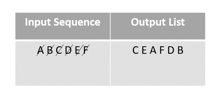
    Then F is selected from the remaining elements in the input sequence and added to the output after marking it visited.

    F_selected

    Step 6

    The next element chosen to add onto the random permutation is D. It is marked and added to the output array.

    output_array

    Step 7

    The last element present in the input list would be B, so it is marked and added onto the output list finally.

    input_list_B

    Modern Method Example

    In order to reduce time complexity of the original method, the modern algorithm is introduced. The modern method uses swapping to shuffle the sequences for example, the algorithm works like shuffling a pack of cards by swapping their places in the original deck. Let us look at an example to understand how modern version of the Fisher-Yates algorithm works.

    Step 1

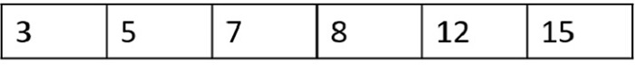
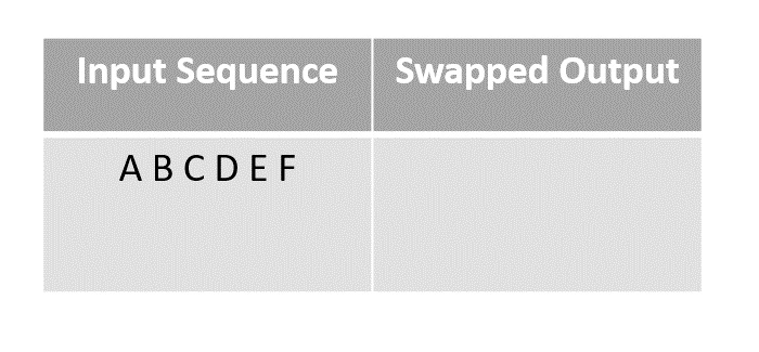
    Consider first few letters of the alphabet as an input and shuffle them using the modern method.
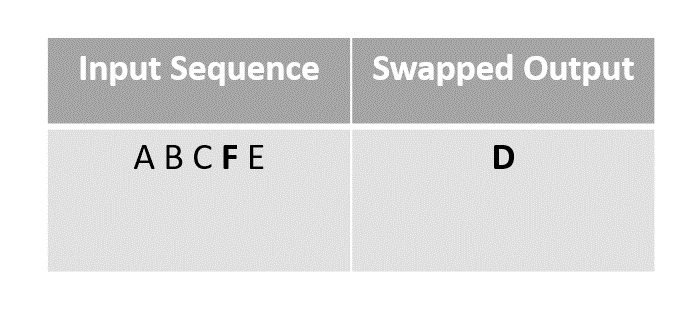
    modern_method

    Step 2

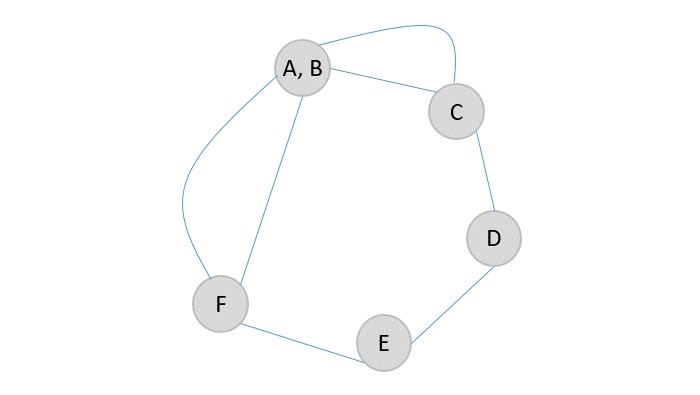
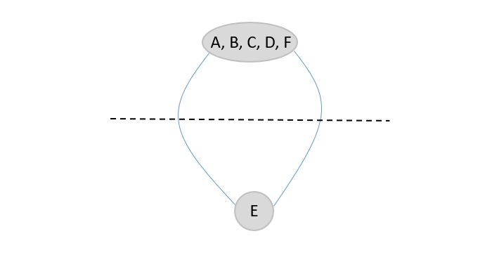
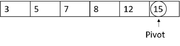
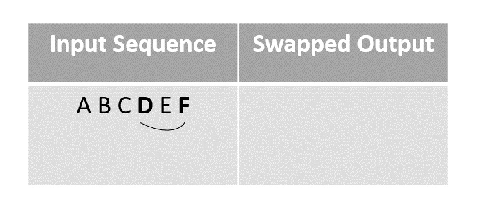
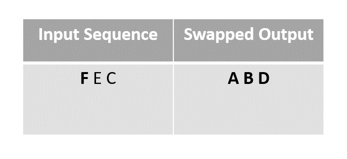
    Randomly choosing the element D and swapping it with the last unmarked element in the sequence, in this case F.
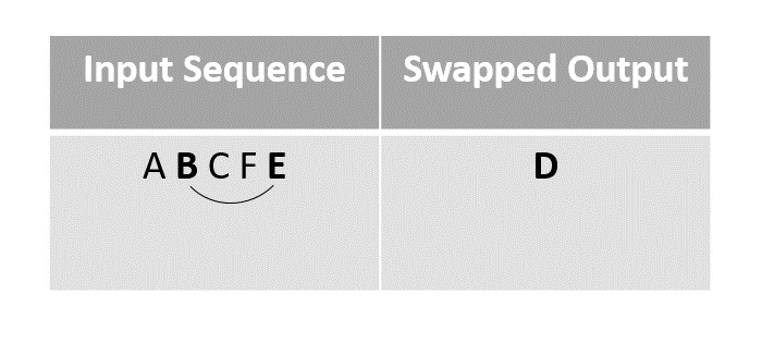
    swapped_output
    choosing_D

    Step 3

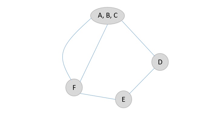
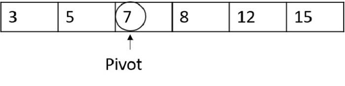
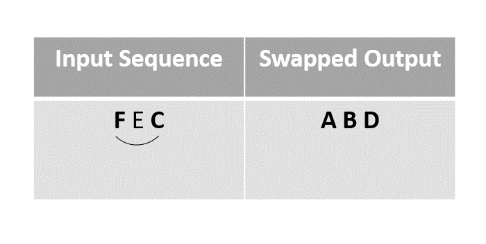
    For the next step we choose element B to swap with the last unmarked element E since F had been moved to Ds place after swapping in the previous step.
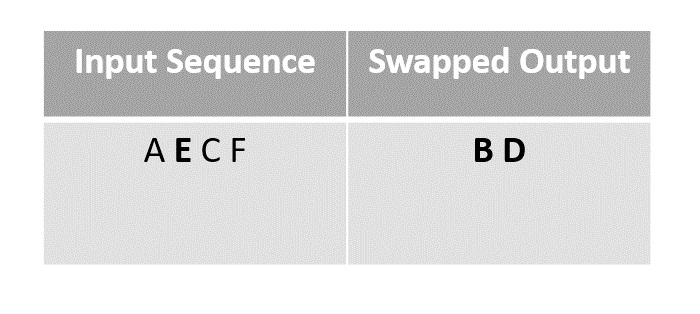
    choose_element_B
    choosed_element_B

    Step 4

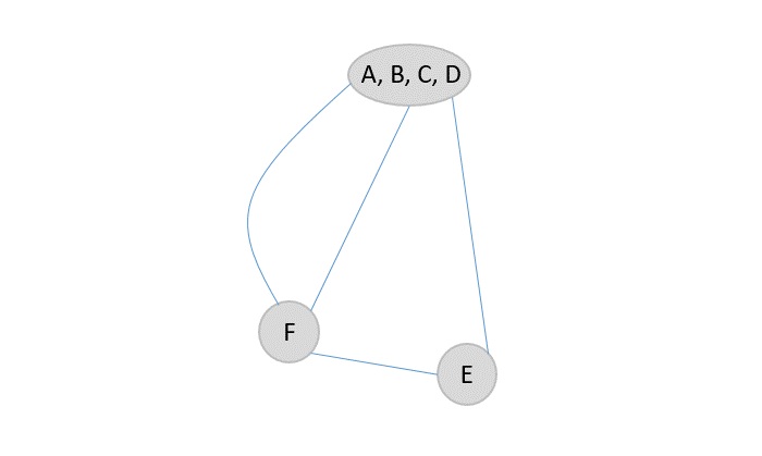
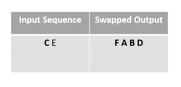
    We next swap the element A with F, since it is the last unmarked element in the list.
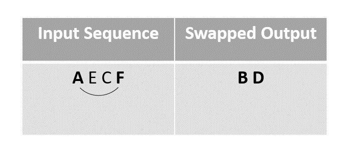
    swap_A_with_F
    last_unmarked_element

    Step 5

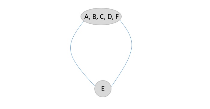
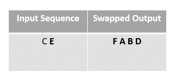
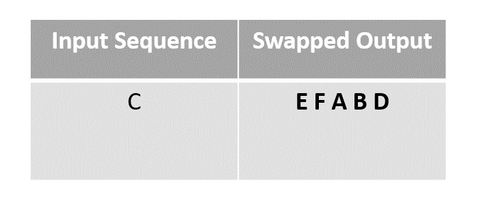
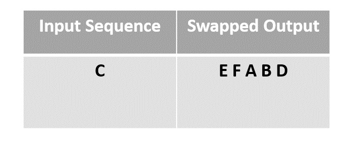
    Then the element F is swapped with the last unmarked element C.

    F_swapped_C
    unmarked_element_C

    Step 6

    The remaining elements in the sequence could be swapped finally, but since the random function chose E as the element it is left as it is.

    chose_E
    chosed_E

    Step 7

    The remaining element C is left as it is without swapping.

    C_left
    final_output_array

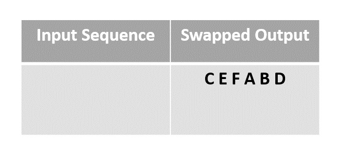
    The array obtained after swapping is the final output array.

    Example

    Following are the implementations of the above approach in various programming langauges −

    CC++JavaPython

    #include <stdio.h>#include <stdlib.h>#include <time.h>// Function to perform Fisher-Yates Shuffle using the original methodvoidfisherYatesShuffle(char arr[],char n){char output[n];// Create an output array to store the shuffled elementschar visited[n];// Create a boolean array to keep track of visited elements// Initialize the visited array with zeros (false)for(char i =0; i < n; i++){
            visited[i]=0;}// Perform the shuffle algorithmfor(char i =0; i < n; i++){char j =rand()% n;// Generate a random index in the input arraywhile(visited[j]){// Find the next unvisited index
                j =rand()% n;}
            output[i]= arr[j];// Add the element at the chosen index to the output array
            visited[j]=1;// Mark the element as visited}// Copy the shuffled elements back to the original arrayfor(char i =0; i < n; i++){
            arr[i]= output[i];}}intmain(){char arr[]={'A','B','C','D','E','F'};char n =sizeof(arr)/sizeof(arr[0]);srand(time(NULL));// Seed the random number generator with the current timefisherYatesShuffle(arr, n);// Call the shuffle functionprintf("Shuffled array: ");for(char i =0; i < n; i++){printf("%c ", arr[i]);// Print the shuffled array}printf("\n");return0;}

    Output

    Shuffled array: A B F D E C 
  • Kargers Minimum Cut Algorithm

    Considering the real-world applications like image segmentation where objects that are focused by the camera need to be removed from the image. Here, each pixel is considered as a node and the capacity between these pixels is reduced. The algorithm that is followed is the minimum cut algorithm.

    Minimum Cut is the removal of minimum number of edges in a graph (directed or undirected) such that the graph is divided into multiple separate graphs or disjoint set of vertices.

    Let us look at an example for a clearer understanding of disjoint sets achieved

    disjoint_sets

    Edges {A, E} and {F, G} are the only ones loosely bonded to be removed easily from the graph. Hence, the minimum cut for the graph would be 2.

    minimum_cut

    The resultant graphs after removing the edges A → E and F → G are {A, B, C, D, G} and {E, F}.

    removing_edges

    Kargers Minimum Cut algorithm is a randomized algorithm to find the minimum cut of a graph. It uses the monte carlo approach so it is expected to run within a time constraint and have a minimal error in achieving output. However, if the algorithm is executed multiple times the probability of the error is reduced. The graph used in kargers minimum cut algorithm is undirected graph with no weights.

    Kargers Minimum Cut Algorithm

    The kargers algorithm merges any two nodes in the graph into one node which is known as a supernode. The edge between the two nodes is contracted and the other edges connecting other adjacent vertices can be attached to the supernode.

    Algorithm

    Step 1 − Choose any random edge [u, v] from the graph G to be contracted.

    Step 2 − Merge the vertices to form a supernode and connect the edges of the other adjacent nodes of the vertices to the supernode formed. Remove the self nodes, if any.

    Step 3 − Repeat the process until theres only two nodes left in the contracted graph.

    Step 4 − The edges connecting these two nodes are the minimum cut edges.

    The algorithm does not always the give the optimal output so the process is repeated multiple times to decrease the probability of error.

    Pseudocode

    Kargers_MinCut(edge, V, E):
       v = V
       while(v > 2):
          i=Random integer in the range [0, E-1]
          s1=find(edge[i].u)
          s2=find(edge[i].v)
          if(s1 != s2):
             v = v-1
             union(u, v)
       mincut=0
       for(i in the range 0 to E-1):
          s1=find(edge[i].u)
          s2=find(edge[i].v)
          if(s1 != s2):
             mincut = mincut + 1
       return mincut
    

    Example

    Applying the algorithm on an undirected unweighted graph G {V, E} where V and E are sets of vertices and edges present in the graph, let us find the minimum cut −

    undirected_unweighted

    Step 1

    Choose any edge, say A → B, and contract the edge by merging the two vertices into one supernode. Connect the adjacent vertex edges to the supernode. Remove the self loops, if any.

    merging_two_vertices

    Step 2

    Contract another edge (A, B) → C, so the supernode will become (A, B, C) and the adjacent edges are connected to the newly formed bigger supernode.

    bigger_supernode

    Step 3

    The node D only has one edge connected to the supernode and one adjacent edge so it will be easier to contract and connect the adjacent edge to the new supernode formed.

    new_supernode_formed

    Step 4

    Among F and E vertices, F is more strongly bonded to the supernode, so the edges connecting F and (A, B, C, D) are contracted.

    F_strongly_bonded_supernode

    Step 5

    Since there are only two nodes present in the graph, the number of edges are the final minimum cut of the graph. In this case, the minimum cut of given graph is 2.

    minimum_cut_graph

    The minimum cut of the original graph is 2 (E → D and E → F).

    Implementation

    Following are the implementations of the above approach in various programming langauges −

    CC++JavaPython

    #include <stdio.h>#include <stdlib.h>#include <time.h>structEdge{int u, v;};structGraph{int V;structEdge* edges;};structGraph*createGraph(int V,int E){structGraph* graph =(structGraph*)malloc(sizeof(structGraph));
        graph->V = V;
        graph->edges =(structEdge*)malloc(E *sizeof(structEdge));return graph;}intfind(int parent[],int i){if(parent[i]== i)return i;returnfind(parent, parent[i]);}voidunionSets(int parent[],int rank[],int x,int y){int xroot =find(parent, x);int yroot =find(parent, y);if(rank[xroot]< rank[yroot])
            parent[xroot]= yroot;elseif(rank[xroot]> rank[yroot])
            parent[yroot]= xroot;else{
            parent[yroot]= xroot;
            rank[xroot]++;}}intkargerMinCut(structGraph* graph){int V = graph->V;int E = V *(V -1)/2;structEdge* edges = graph->edges;int* parent =(int*)malloc(V *sizeof(int));int* rank =(int*)malloc(V *sizeof(int));for(int i =0; i < V; i++){
            parent[i]= i;
            rank[i]=0;}int v = V;while(v >2){int randomIndex =rand()% E;int u = edges[randomIndex].u;int w = edges[randomIndex].v;int setU =find(parent, u);int setW =find(parent, w);if(setU != setW){
                v--;unionSets(parent, rank, setU, setW);}
            edges[randomIndex]= edges[E -1];
            E--;}int minCut =0;for(int i =0; i < E; i++){int setU =find(parent, edges[i].u);int setW =find(parent, edges[i].v);if(setU != setW)
                minCut++;}free(parent);free(rank);return minCut;}intmain(){int V =4;int E =5;structGraph* graph =createGraph(V, E);
        graph->edges[0].u =0;
        graph->edges[0].v =1;
        graph->edges[1].u =0;
        graph->edges[1].v =2;
        graph->edges[2].u =0;
        graph->edges[2].v =3;
        graph->edges[3].u =1;
        graph->edges[3].v =3;
        graph->edges[4].u =2;
        graph->edges[4].v =3;srand(time(NULL));int minCut =kargerMinCut(graph);printf("Minimum Cut: %d\n", minCut);free(graph->edges);free(graph);return0;}

    Output

    Minimum Cut: 2
  • Randomized Quick Sort Algorithm

    Quicksort is a popular sorting algorithm that chooses a pivot element and sorts the input list around that pivot element. To learn more about quick sort, please click here.

    Randomized quick sort is designed to decrease the chances of the algorithm being executed in the worst case time complexity of O(n2). The worst case time complexity of quick sort arises when the input given is an already sorted list, leading to n(n 1) comparisons. There are two ways to randomize the quicksort −

    • Randomly shuffling the inputs: Randomization is done on the input list so that the sorted input is jumbled again which reduces the time complexity. However, this is not usually performed in the randomized quick sort.
    • Randomly choosing the pivot element: Making the pivot element a random variable is commonly used method in the randomized quick sort. Here, even if the input is sorted, the pivot is chosen randomly so the worst case time complexity is avoided.

    Randomized Quick Sort Algorithm

    The algorithm exactly follows the standard algorithm except it randomizes the pivot selection.

    Pseudocode

    partition-left(arr[], low, high)
       pivot = arr[high]
       i = low // place for swapping
       for j := low to high  1 do
          if arr[j] <= pivot then
             swap arr[i] with arr[j]
             i = i + 1
       swap arr[i] with arr[high]
       return i
    
    partition-right(arr[], low, high)
       r = Random Number from low to high
       Swap arr[r] and arr[high]
       return partition-left(arr, low, high)
    
    quicksort(arr[], low, high)
       if low < high
          p = partition-right(arr, low, high)
          quicksort(arr, low , p-1)
          quicksort(arr, p+1, high)
    

    Example

    Let us look at an example to understand how randomized quicksort works in avoiding the worst case time complexity. Since, we are designing randomized algorithms to decrease the occurrence of worst cases in time complexity lets take a sorted list as an input for this example.

    The sorted input list is 3, 5, 7, 8, 12, 15. We need to apply the quick sort algorithm to sort the list.

    sorted_input_list

    Step 1

    Considering the worst case possible, if the random pivot chosen is also the highest index number, it compares all the other numbers and another pivot is selected.

    pivot

    Since 15 is greater than all the other numbers in the list, it wont be swapped, and another pivot is chosen.

    Step 2

    This time, if the random pivot function chooses 7 as the pivot number −

    pivot_7

    Now the pivot divides the list into half so standard quick sort is carried out usually. However, the time complexity is decreased than the worst case.

    It is to be noted that the worst case time complexity of the quick sort will always remain O(n2) but with randomizations we are decreasing the occurrences of that worst case.

    Implementation

    Following are the implementations of the above approach in various programming langauges −

    CC++JavaPython

    #include <stdio.h>#include <stdlib.h>#include <time.h>// Function to swap two elementsvoidswap(int* a,int* b){int t =*a;*a =*b;*b = t;}// Function to partition the arrayintpartition_left(int arr[],int low,int high){int pivot = arr[high];int i = low;for(int j = low; j < high; j++){if(arr[j]<= pivot){swap(&arr[i],&arr[j]);
                i++;}}swap(&arr[i],&arr[high]);return i;}// Function to perform random partitionintpartition_right(int arr[],int low,int high){srand(time(NULL));int r = low +rand()%(high - low);swap(&arr[r],&arr[high]);returnpartition_left(arr, low, high);}// Recursive function for quicksortvoidquicksort(int arr[],int low,int high){if(low < high){int p =partition_right(arr, low, high);quicksort(arr, low, p -1);quicksort(arr, p +1, high);}}// Function to print the arrayvoidprintArray(int arr[],int size){for(int i =0; i < size; i++)printf("%d ", arr[i]);printf("\n");}// Driver codeintmain(){int arr[]={6,4,12,8,15,16};int n =sizeof(arr)/sizeof(arr[0]);printf("Original array: ");printArray(arr, n);quicksort(arr,0, n -1);printf("Sorted array: ");printArray(arr, n);return0;}

    Output

    Original array: 6 4 12 8 15 16 
    Sorted array: 4 6 8 12 15 16
  • Randomized Algorithms

    Randomized algorithm is a different design approach taken by the standard algorithms where few random bits are added to a part of their logic. They are different from deterministic algorithms; deterministic algorithms follow a definite procedure to get the same output every time an input is passed where randomized algorithms produce a different output every time theyre executed. It is important to note that it is not the input that is randomized, but the logic of the standard algorithm.

    Deterministic_Algorithm

    Figure 1: Deterministic Algorithm

    Unlike deterministic algorithms, randomized algorithms consider randomized bits of the logic along with the input that in turn contribute towards obtaining the output.

    Randomized_Algorithms

    Figure 2: Randomized Algorithm

    However, the probability of randomized algorithms providing incorrect output cannot be ruled out either. Hence, the process called amplification is performed to reduce the likelihood of these erroneous outputs. Amplification is also an algorithm that is applied to execute some parts of the randomized algorithms multiple times to increase the probability of correctness. However, too much amplification can also exceed the time constraints making the algorithm ineffective.

    Classification of Randomized Algorithms

    Randomized algorithms are classified based on whether they have time constraints as the random variable or deterministic values. They are designed in their two common forms − Las Vegas and Monte Carlo.

    Classification_Randomized_Algorithms
    • Las Vegas − The Las Vegas method of randomized algorithms never gives incorrect outputs, making the time constraint as the random variable. For example, in string matching algorithms, las vegas algorithms start from the beginning once they encounter an error. This increases the probability of correctness. Eg., Randomized Quick Sort Algorithm.
    • Monte Carlo − The Monte Carlo method of randomized algorithms focuses on finishing the execution within the given time constraint. Therefore, the running time of this method is deterministic. For example, in string matching, if monte carlo encounters an error, it restarts the algorithm from the same point. Thus, saving time. Eg., Kargers Minimum Cut Algorithm

    Need for Randomized Algorithms

    This approach is usually adopted to reduce the time complexity and space complexity. But there might be some ambiguity about how adding randomness will decrease the runtime and memory stored, instead of increasing; we will understand that using the game theory.

    The Game Theory and Randomized Algorithms

    The basic idea of game theory actually provides with few models that help understand how decision-makers in a game interact with each other. These game theoretical models use assumptions to figure out the decision-making structure of the players in a game. The popular assumptions made by these theoretical models are that the players are both rational and take into account what the opponent player would decide to do in a particular situation of a game. We will apply this theory on randomized algorithms.

    Zero-sum game

    The zero-sum game is a mathematical representation of the game theory. It has two players where the result is a gain for one player while it is an equivalent loss to the other player. So, the net improvement is the sum of both players status which sums up to zero.

    Randomized algorithms are based on the zero-sum game of designing an algorithm that gives lowest time complexity for all inputs. There are two players in the game; one designs the algorithm and the opponent provides with inputs for the algorithm. The player two needs to give the input in such a way that it will yield the worst time complexity for them to win the game. Whereas, the player one needs to design an algorithm that takes minimum time to execute any input given.

    For example, consider the quick sort algorithm where the main algorithm starts from selecting the pivot element. But, if the player in zero-sum game chooses the sorted list as an input, the standard algorithm provides the worst case time complexity. Therefore, randomizing the pivot selection would execute the algorithm faster than the worst time complexity. However, even if the algorithm chose the first element as pivot randomly and obtains the worst time complexity, executing it another time with the same input will solve the problem since it chooses another pivot this time.

    On the other hand, for algorithms like merge sort the time complexity does not depend on the input; even if the algorithm is randomized the time complexity will always remain the same. Hence, randomization is only applied on algorithms whose complexity depends on the input.

    Examples

    Few popular examples of the Randomized algorithms are −

    • Randomized Quick Sort Algorithm
    • Kargers Minimum Cut Algorithm
    • Fisher-Yates Shuffle Algorithm
    • The Subset Sum Problem