Category: Statistics for Machine Learning

In machine learning, a hypothesis is a proposed explanation or solution for a problem. It is a tentative assumption or idea that can be tested and validated using data. In supervised learning, the hypothesis is the model that the algorithm is trained on to make predictions on unseen data.

Hypothesis in machine learning is generally expressed as a function that maps input data to output predictions. In other words, it defines the relationship between the input and output variables. The goal of machine learning is to find the best possible hypothesis that can generalize well to unseen data.

What is Hypothesis?

A hypothesis is an assumption or idea used as a possible explanation for something that can be tested to see if it might be true. The hypothesis is generally based on some evidence. A simple example of a hypothesis will be the assumption: “The price of a house is directly proportional to its square footage”.

Hypothesis in Machine Learning

In machine learning, mainly supervised learning, a hypothesis is generally expressed as a function that maps input data to output predictions. In other words, it defines the relationship between the input and output variables. The goal of machine learning is to find the best possible hypothesis that can generalize well to unseen data.

In supervised learning, a hypothesis (h) can be represented mathematically as follows −

h(x)=ŷ 

Here x is input and ŷ is predicted value.

Hypothesis Function (h)

A machine learning model is defined by its hypothesis function. A hypothesis function is a mathematical function that takes input and returns output. For a simple linear regression problem, a hypothesis can be represented as a linear function of the input feature (‘x’).

h(x)=w0+w1x

Where w₀ and w₁ are the parameters (weights) and ‘x’ is the input feature.

For a multiple linear regression problem, the model can be represented mathematically as follows −

h(x)=w0+w1x+…+wnxn

Where,

• w₀, w₁, …, w_n are the parameters.
• x₁, x₂, …, x_n are the input data (features)
• n is the total number of training examples
• h(x) is hypothesis function

The machine learning process tries to find the optimal values for the parameters such that it minimizes the cost function.

Hypothesis Space (H)

A Set of all possible hypotheses is known as a hypotheses space or set. The machine learning process tries to find the best-fit hypothesis among all possible hypotheses.

For a linear regression model, the hypothesis includes all possible linear functions.

The process of finding the best hypothesis is called model training or learning. During the training process, the algorithm adjusts the model parameters to minimize the error or loss function, which measures the difference between the predicted output and the actual output.

Types of Hypothesis in Machine Learning

There are mainly two types of hypotheses in machine learning −

1. Null Hypothesis (H₀)

The null hypothesis is the default assumption or explanation that there is no relation between input features and output variables. In the machine learning process, we try to reject the null hypothesis in favor of another hypothesis. The null hypothesis is rejected if the “p-value” is less than the significance level (α)

2. Alternative Hypothesis (H₁)

The alternate hypothesis is a direct contradiction of the null hypothesis. The alternative hypothesis is a hypothesis that assumes a significant relation between the input data and output (target value). When we reject the null hypothesis, we accept an alternative hypothesis. When the p-value is less than the significance level, we reject the null hypothesis and accept the alternative hypothesis.

Hypothesis Testing in Machine Learning

Hypothesis testing determines whether the data sufficiently supports a particular hypothesis. The following are steps involved in hypothesis testing in machine learning −

• State the null and alternative hypotheses − define null hypothesis H₀ and alternative hypothesis H₁.
• Choose a significance level (α) − The significance level is the probability of rejecting a null hypothesis when it is true. Generally, the value of α is 0.05 (5%) or 0.01 (1%).
• Calculate a test statistic − Calculate t-statistic or z-statistic based on data and type of hypothesis.
• Determine the p-value − The p-value measures the strength against null hypothesis. If the p-value is less than the significance level, reject the null hypothesis.
• Make a decision − small p-value indicates that there are significant relations between the features and target variables. Reject the null hypothesis.

How to Find the Best Hypothesis?

The process of finding the best hypothesis is called model training or learning. During the training process, the algorithm adjusts the model parameters to minimize the error or loss function, which measures the difference between the predicted output and the actual output.

Optimization techniques such as gradient descent are used to find the best hypothesis. The best hypothesis is one that minimizes the cost function or error function.

For example, in linear regression, the Mean Square Error (MSE) is used as a cost function (J(w)). It is defined as

J(x)=12n∑i=0n(h(xi)−yi)2

Where,

• h(x_i) is the predicted output for the i^th data sample or observation..
• y_i is the actual target value for the i^th sample.
• n is the number of training data.

Here, the goal is to find the optimal values of w that minimize the cost function. The hypothesis represented using these optimal values of parameters w will be the best hypothesis.

Properties of a Good Hypothesis

The hypothesis plays a critical role in the success of a machine learning model. A good hypothesis should have the following properties −

• Generalization − The model should be able to make accurate predictions on unseen data.
• Simplicity − The model should be simple and interpretable so that it is easier to understand and explain.
• Robustness − The model should be able to handle noise and outliers in the data.
• Scalability − The model should be able to handle large amounts of data efficiently.

There are many types of machine learning algorithms that can be used to generate hypotheses, including linear regression, logistic regression, decision trees, support vector machines, neural networks, and more.

Once the model is trained, it can be used to make predictions on new data. However, it is important to evaluate the performance of the model before using it in the real world. This is done by testing the model on a separate validation set or using cross-validation techniques.

Bias and variance are two important concepts in machine learning that describe the sources of error in a model’s predictions. Bias refers to the error that results from oversimplifying the underlying relationship between the input features and the output variable. At the same time, variance refers to the error that results from being too sensitive to fluctuations in the training data.

In machine learning, we strive to minimize both bias and variance in order to build a model that can accurately predict on unseen data. A high-bias model may be too simplistic and underfit the training data. In contrast, a model with high variance may overfit the training data and fail to generalize to new data.

Generally, a machine learning model shows three types of error – bias, variance, and irreducible error. There is a tradeoff between bias and variance errors. Decreasing the bias leads to increasing the variance and vice versa.

What is Bias?

Bias is calculated as the difference between average prediction and actual value. In machine learning, bias (systematic error) occurs when a model makes incorrect assumptions about data.

A model with high bias does not match well training data as well as test data. It leads to high errors in training and test data.

While the model with low bias matches the training data well (high training accuracy or less error in training). It leads to low error in training data but high error in test data.

Types of Bias

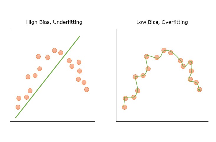
• High Bias − High bias occurs due to erroneous assumptions in the machine learning model. Models with high bias cannot capture the hidden pattern in the training data. This leads to underfitting.his leads to underfitting. Features of high bias are a highly simplified model, underfitting, and high error in training and test data.
• Low Bias − Models with low bias can capture the hidden pattern in the training data. Low bias leads to high variance and, eventually, overfitting. Low bias generally occurs due to the ML model being overly complex.

Below figure shows pictorial representation of the high and low bias error.

Example of Bias in Models

A linear regression model trying to fit the non-linear data will show a high bias. Some examples of models with high bias are linear regression and logistic regression. Some examples of models with low bias are decision trees, k-nearest neighbors, and support vector machines.

Impact of Bias on Model Performance

High bias can lead to poor performance on both training and test datasets. High-bias models will not be able to generalize on the new, unseen data.

What is Variance?

Variance is a measure of the spread or dispersion of numbers in a given set of observations with respect to the mean. It basically measures how a set of numbers is spread out from the average. In statistics and probability, variance is defined as the expectation of the squared deviation of a random variable from the sample mean.

In machine learning, variance is the variability of model prediction on different datasets. The variance shows how much model prediction varies when there is a slight variation in data. If model accuracies on training and test data vary greatly, the model has high variance.

A model with high variance can even fit noises on training data but lacks generalization to new, unseen data.

Types of Variance

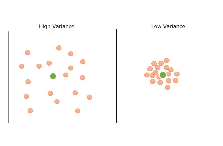
• High Variance − High variance models capture noise along with hidden pattern. It leads to overfitting. High variance models show high training accuracy but low test accuracy. Some features of a high variance model are an overly complex model, overfitting, low error on training data, and high error or test data.
• Low Variance − A model with low variance is unable to capture the hidden pattern in the data. Low variance may occur when we have a very small amount of data or use a very simplified model. Low variance leads to underfitting.

Below figure shows pictorial representation of the high and low variance examples.

Example of Variance in Models

A decision tree with many branches that fits the training data perfectly but does not fit properly on test data is an example of high variance. Examples of high variance: k-nearest neighbors, decision trees, and support vector machines (SVMs).

Impact of Variance on Model Performance

A high variance can lead to a model that performs well with training data but fails to perform well on training data. During training, high-variance models fit the training data so well that they even capture the noises as actual patterns. Models with high variance errors are known as overfitting models.

Bias-Variance Tradeoff

The bias-variance tradeoff is finding a balance between the error introduced by bias and the error introduced by variance. With increased model complexity, the bias will decrease, but the variance will increase. However, when we decrease the model complexity, the bias will increase, and the variance will decrease. So we need a balance between bias and variance so total prediction error is minimized.

A machine learning model will not perform well on new, unseen data if it has a high bias or variance in training. A good model should not have either high bias or variance. We can’t reduce both bias and variance at the same time. When bias reduces, variance will increase. So we need to find an optimal bias and variance such that the prediction error is minimized.

In machine learning, bias-variance tradeoff is important because a model with high bias or high.

Graphical Representation

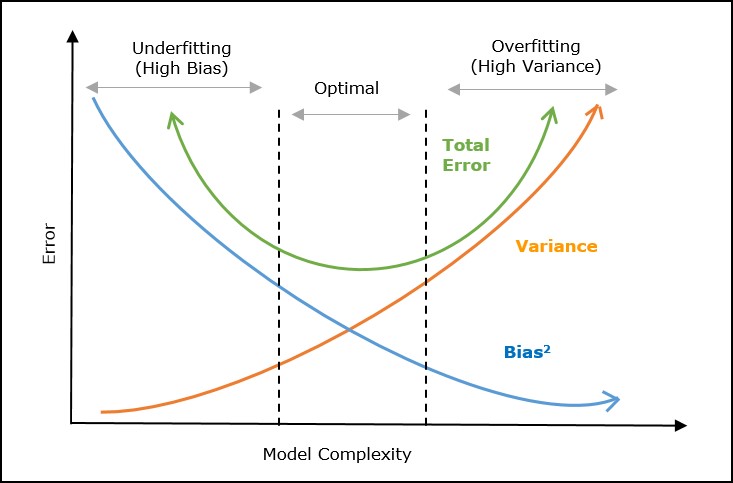
The following graph represents the tradeoff between bias and variance graphically.

In the above graph, the X-axis represents the model complexity, and the Y-axis represents the prediction error. The total error is the sum of bias error and variance error. The optimal region shows the area with the balance between bias and variance, showing optimal model complexity with minimum error.

Mathematical Representation

The prediction error in the machine learning model can be written mathematically as follows −

Error = bias² + variance + irreducible error.

To minimize the model prediction error, we need to choose model complexity in such a way so that a balance between these two errors can be met.

The main objective of the bias-variance tradeoff is to find optimal values of bias and variance (model complexity) that minimize the error.

Techniques to Balance Bias and Variance

There are different techniques to balance bias and variance to achieve an optimal prediction error.

1. Reducing High Bias

• Choosing a more complex model − As we have seen in the above diagram, choosing a more complex model may reduce the bias error of the model prediction.
• Adding more features − Adding mode features can increase the complexity of the model that can capture even better hidden patterns that will decrease the bias error of the model.
• Reducing regularization − Regularization prevents overfitting, but while decreasing the variance, it can increase bias. So, reducing the regularization parameters or removing regularization overall can reduce bias errors.

2. Reducing High Variance

• Applying regularization techniques − Regularization techniques add penalty to complex model that will eventually result in reduced complexity of the model. A less complex model will show less variance.
• Simplifying model complexity − A less complex model will have low variance. You can reduce the variance by using a simpler algorithm.
• Adding more data − Adding more data to the dataset can help the model to perform better showing less variance.
• Cross-validation − Cross-validation can be useful to identify overfitting by comparing the performance on training and validation sets of the datasets.

Bias and Variance Examples Using Python

Let’s implement some practical examples using Python programming language. We have provided here four examples. The first three examples show some level of high/ low bias or variance. The fourth example shows the optimal value of both bias and variance.

Example of High Bias

Below is an implementation example in Python that illustrates how bias and variance can be analyzed using the Boston Housing dataset −

import numpy as np
import pandas as pd
from sklearn.datasets import load_boston

boston = load_boston()
X = boston.data
y = boston.target
from sklearn.model_selection import train_test_split

X_train, X_test, y_train, y_test = train_test_split(X, y, test_size=0.2,
random_state=42)from sklearn.linear_model import LinearRegression
from sklearn.metrics import mean_squared_error

lr = LinearRegression()
lr.fit(X_train, y_train)

train_preds = lr.predict(X_train)
train_mse = mean_squared_error(y_train, train_preds)print("Training MSE:", train_mse)

test_preds = lr.predict(X_test)
test_mse = mean_squared_error(y_test, test_preds)print("Testing MSE:", test_mse)

Output

The output shows the training and testing mean squared errors (MSE) of the linear regression model. The training MSE is 21.64 and the testing MSE is 24.29, indicating that the model has a high level of bias and moderate variance.

Training MSE: 21.641412753226312
Testing MSE: 24.291119474973456

Example of Low Bias and High Variance

Let’s try a polynomial regression model −

from sklearn.preprocessing import PolynomialFeatures

poly = PolynomialFeatures(degree=2)
X_train_poly = poly.fit_transform(X_train)
X_test_poly = poly.transform(X_test)

pr = LinearRegression()
pr.fit(X_train_poly, y_train)

train_preds = pr.predict(X_train_poly)
train_mse = mean_squared_error(y_train, train_preds)print("Training MSE:", train_mse)

test_preds = pr.predict(X_test_poly)
test_mse = mean_squared_error(y_test, test_preds)print("Testing MSE:", test_mse)

Output

The output shows the training and testing MSE of the polynomial regression model with degree=2. The training MSE is 5.31 and the testing MSE is 14.18, indicating that the model has a lower bias but higher variance compared to the linear regression model.

Training MSE: 5.31446956670908
Testing MSE: 14.183558207567042

Example of Low Variance

To reduce variance, we can use regularization techniques such as ridge regression or lasso regression. In the following example, we will be using ridge regression −

from sklearn.linear_model import Ridge

ridge = Ridge(alpha=1)
ridge.fit(X_train_poly, y_train)

train_preds = ridge.predict(X_train_poly)
train_mse = mean_squared_error(y_train, train_preds)print("Training MSE:", train_mse)

test_preds = ridge.predict(X_test_poly)
test_mse = mean_squared_error(y_test, test_preds)print("Testing MSE:", test_mse)

Output

The output shows the training and testing MSE of the ridge regression model with alpha=1. The training MSE is 9.03 and the testing MSE is 13.88 compared to the polynomial regression model, indicating that the model has a lower variance but slightly higher bias.

Training MSE: 9.03220937860839
Testing MSE: 13.882093755326755

Example of Optimal Bias and Variance

We can further tune the hyperparameter alpha to find the optimal balance between bias and variance. Let’s see an example −

from sklearn.model_selection import GridSearchCV

param_grid ={'alpha': np.logspace(-3,3,7)}
ridge_cv = GridSearchCV(Ridge(), param_grid, cv=5)
ridge_cv.fit(X_train_poly, y_train)

train_preds = ridge_cv.predict(X_train_poly)
train_mse = mean_squared_error(y_train, train_preds)print("Training MSE:", train_mse)

test_preds = ridge_cv.predict(X_test_poly)
test_mse = mean_squared_error(y_test, test_preds)print("Testing MSE:", test_mse)

Output

The output shows the training and testing MSE of the ridge regression model with the optimal alpha value.

Training MSE: 8.326082686584716
Testing MSE: 12.873907256619141

The training MSE is 8.32 and the testing MSE is 12.87, indicating that the model has a good balance between bias and variance.

Skewness and kurtosis are two important measures of the shape of a probability distribution in machine learning.

Skewness refers to the degree of asymmetry of a distribution. A distribution is said to be skewed if it is not symmetrical about its mean. Skewness can be positive, indicating that the tail of the distribution is longer on the right-hand side, or negative, indicating that the tail of the distribution is longer on the left-hand side. A skewness of zero indicates that the distribution is perfectly symmetrical.

Kurtosis refers to the degree of peakedness of a distribution. A distribution with high kurtosis has a sharper peak and heavier tails than a normal distribution, while a distribution with low kurtosis has a flatter peak and lighter tails. Kurtosis can be positive, indicating a higher-than-normal peak, or negative, indicating a lower than normal peak. A kurtosis of zero indicates a normal distribution.

Both skewness and kurtosis can have important implications for machine learning algorithms, as they can affect the assumptions of the models and the accuracy of the predictions. For example, a highly skewed distribution may require data transformation or the use of non-parametric methods, while a highly kurtotic distribution may require different statistical models or more robust estimation methods.

Example

In Python, the SciPy library provides functions for calculating skewness and kurtosis of a dataset. For example, the following code calculates the skewness and kurtosis of a dataset using the skew() and kurtosis() functions −

import numpy as np
from scipy.stats import skew, kurtosis

# Generate a random dataset
data = np.random.normal(0,1,1000)# Calculate the skewness and kurtosis of the dataset
skewness = skew(data)
kurtosis = kurtosis(data)# Print the resultsprint('Skewness:', skewness)print('Kurtosis:', kurtosis)

This code generates a random dataset of 1000 samples from a normal distribution with mean 0 and standard deviation 1. It then calculates the skewness and kurtosis of the dataset using the skew() and kurtosis() functions from the SciPy library. Finally, it prints the results to the console.

Output

On executing this code, you will get the following output −

Skewness: -0.04119418903611285
Kurtosis: -0.1152250196054534

The resulting skewness and kurtosis values should be close to zero for a normal distribution.

In machine learning, data distribution refers to the way in which data points are distributed or spread out across a dataset. It is important to understand the distribution of data in a dataset, as it can have a significant impact on the performance of machine learning algorithms.

Data distribution can be characterized by several statistical measures, including mean, median, mode, standard deviation, and variance. These measures help to describe the central tendency, spread, and shape of the data.

Some common types of data distribution in machine learning are given below −

Normal Distribution

Normal distribution, also known as Gaussian distribution, is a continuous probability distribution that is widely used in machine learning and statistics. It is a bell-shaped curve that describes the probability distribution of a random variable that is symmetric around the mean. The normal distribution has two parameters, the mean (μ) and the standard deviation (σ).

In machine learning, normal distribution is often used to model the distribution of error terms in linear regression and other statistical models. It is also used as a basis for various hypothesis tests and confidence intervals.

One important property of normal distribution is the empirical rule, also known as the 68- 95-99.7 rule. This rule states that approximately 68% of the observations fall within one standard deviation of the mean, 95% of the observations fall within two standard deviations of the mean, and 99.7% of the observations fall within three standard deviations of the mean.

Python provides various libraries that can be used to work with normal distributions. One such library is scipy.stats, which provides functions for calculating the probability density function (PDF), cumulative distribution function (CDF), percent point function (PPF), and random variables for normal distribution.

Example

Here is an example of using scipy.stats to generate and visualize a normal distribution −

import numpy as np
from scipy.stats import norm
import matplotlib.pyplot as plt

# Generate a random sample of 1000 values from a normal distribution
mu =0# Mean
sigma =1# Standard deviation
sample = np.random.normal(mu, sigma,1000)# Calculate the PDF for the normal distribution
x = np.linspace(mu -3*sigma, mu +3*sigma,100)
pdf = norm.pdf(x, mu, sigma)# Plot the histogram of the random sample and the PDF of the normal
distribution
plt.figure(figsize=(7.5,3.5))
plt.hist(sample, bins=30, density=True, alpha=0.5)
plt.plot(x, pdf)
plt.show()

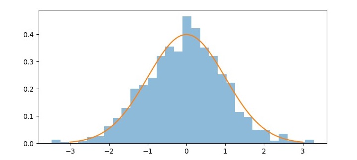
In this example, we first generate a random sample of 1000 values from a normal distribution with mean 0 and standard deviation 1 using np.random.normal. We then use norm.pdf to calculate the PDF for the normal distribution and np.linspace to generate an array of 100 evenly spaced values between μ -3σ and μ +3σ

Finally, we plot the histogram of the random sample using plt.hist and overlay the PDF of the normal distribution using plt.plot.

Output

The resulting plot shows the bell-shaped curve of the normal distribution and the histogram of the random sample that approximates the normal distribution.

Skewed Distribution

A skewed distribution in machine learning refers to a dataset that is not evenly distributed around its mean, or average value. In a skewed distribution, the majority of the data points tend to cluster towards one end of the distribution, with a smaller number of data points at the other end.

There are two types of skewed distributions: left-skewed and right-skewed. A left-skewed distribution, also known as a negative-skewed distribution, has a long tail towards the left side of the distribution, with the majority of data points towards the right side. In contrast, a right-skewed distribution, also known as a positive-skewed distribution, has a long tail towards the right side of the distribution, with the majority of data points towards the left side.

Skewed distributions can occur in many different types of datasets, such as financial data, social media metrics, or healthcare records. In machine learning, it is important to identify and handle skewed distributions appropriately, as they can affect the performance of certain algorithms and models. For example, skewed data can lead to biased predictions and inaccurate results in some cases and may require preprocessing techniques such as normalization or data transformation to improve the performance of the model.

Example

Here is an example of generating and plotting a skewed distribution using Python’s NumPy and Matplotlib libraries −

import numpy as np
import matplotlib.pyplot as plt

# Generate a skewed distribution using NumPy's random function
data = np.random.gamma(2,1,1000)# Plot a histogram of the data to visualize the distribution
plt.figure(figsize=(7.5,3.5))
plt.hist(data, bins=30)# Add labels and title to the plot
plt.xlabel('Value')
plt.ylabel('Frequency')
plt.title('Skewed Distribution')# Show the plot
plt.show()

Output

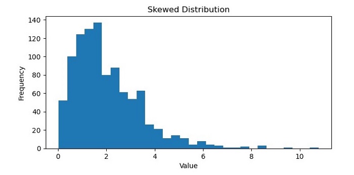
On executing this code, you will get the following plot as the output −

Uniform Distribution

A uniform distribution in machine learning refers to a probability distribution in which all possible outcomes are equally likely to occur. In other words, each value in a dataset has the same probability of being observed, and there is no clustering of data points around a particular value.

The uniform distribution is often used as a baseline for comparison with other distributions, as it represents a random and unbiased sampling of the data. It can also be useful in certain types of applications, such as generating random numbers or selecting items from a set without bias.

In probability theory, the probability density function of a continuous uniform distribution is defined as −

f(x)={10fora≤x≤botherwise

where a and b are the minimum and maximum values of the distribution, respectively. mean of a uniform distribution is a+b2 and the variance is (b−a)212

Example

In Python, the NumPy library provides functions for generating random numbers from a uniform distribution, such as numpy.random.uniform(). These functions take as arguments the minimum and maximum values of the distribution and can be used to generate datasets with a uniform distribution.

Here is an example of generating a uniform distribution using Python’s NumPy library −

import numpy as np
import matplotlib.pyplot as plt

# Generate 10,000 random numbers from a uniform distribution between 0 and 1
uniform_data = np.random.uniform(low=0, high=1, size=10000)# Plot the histogram of the uniform data
plt.figure(figsize=(7.5,3.5))
plt.hist(uniform_data, bins=50, density=True)# Add labels and title to the plot
plt.xlabel('Value')
plt.ylabel('Frequency')
plt.title('Uniform Distribution')# Show the plot
plt.show()

Output

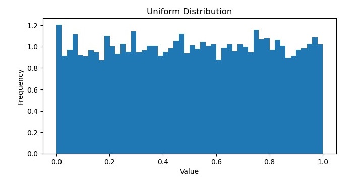
It will produce the following plot as the output −

Bimodal Distribution

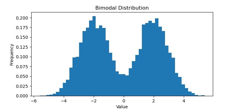
In machine learning, a bimodal distribution is a probability distribution that has two distinct modes or peaks. In other words, the distribution has two regions where the data values are most likely to occur, separated by a valley or trough where the data is less likely to occur.

Bimodal distributions can arise in various types of data, such as biometric measurements, economic indicators, or social media metrics. They can represent different subpopulations within the dataset, or different modes of behavior or trends over time.

Bimodal distributions can be identified and analyzed using various statistical methods, such as histograms, kernel density estimations, or hypothesis testing. In some cases, bimodal distributions can be fitted to specific probability distributions, such as the Gaussian mixture model, which allows for modeling the underlying subpopulations separately.

Example

In Python, libraries such as NumPy, SciPy, and Matplotlib provide functions for generating and visualizing bimodal distributions.

For example, the following code generates and plots a bimodal distribution −

import numpy as np
import matplotlib.pyplot as plt

# Generate 10,000 random numbers from a bimodal distribution
bimodal_data = np.concatenate((np.random.normal(loc=-2, scale=1, size=5000),
   np.random.normal(loc=2, scale=1, size=5000)))# Plot the histogram of the bimodal data
plt.figure(figsize=(7.5,3.5))
plt.hist(bimodal_data, bins=50, density=True)# Add labels and title to the plot
plt.xlabel('Value')
plt.ylabel('Frequency')
plt.title('Bimodal Distribution')# Show the plot
plt.show()

Output

On executing this code, you will get the following plot as the output −

Percentiles are a statistical concept used in machine learning to describe the distribution of a dataset. A percentile is a measure that indicates the value below which a given percentage of observations in a group of observations falls.

For example, the 25th percentile (also known as the first quartile) is the value below which 25% of the observations in the dataset fall, while the 75th percentile (also known as the third quartile) is the value below which 75% of the observations in the dataset fall.

Percentiles can be used to summarize the distribution of a dataset and identify outliers. In machine learning, percentiles are often used in data preprocessing and exploratory data analysis to gain insights into the data.

Python provides several libraries for calculating percentiles, including NumPy and Pandas.

Calculating Percentiles using NumPy

Below is an example of how to calculate percentiles using NumPy −

Example

import numpy as np

data = np.array([1,2,3,4,5])
p25 = np.percentile(data,25)
p75 = np.percentile(data,75)print('25th percentile:', p25)print('75th percentile:', p75)

In this example, we create a sample dataset using NumPy and then calculate the 25th and 75th percentiles using the np.percentile() function.

Output

The output shows the values of the percentiles for the dataset.

25th percentile: 2.0
75th percentile: 4.0

Calculating Percentiles using Pandas

Below is an example of how to calculate percentiles using Pandas −

Example

import pandas as pd

data = pd.Series([1,2,3,4,5])
p25 = data.quantile(0.25)
p75 = data.quantile(0.75)print('25th percentile:', p25)print('75th percentile:', p75)

In this example, we create a Pandas series object and then calculate the 25th and 75th percentiles using the quantile() method of the series object.

Output

The output shows the values of the percentiles for the dataset.

25th percentile: 2.0
75th percentile: 4.0

Standard deviation is a measure of the amount of variation or dispersion of a set of data values around their mean. In machine learning, it is an important statistical concept that is used to describe the spread or distribution of a dataset.

Standard deviation is calculated as the square root of the variance, which is the average of the squared differences from the mean. The formula for calculating standard deviation is as follows −

σ=[Σ(x−μ)2/N]‾‾‾‾‾‾‾‾‾‾‾‾‾√

Where −

• σis the standard deviation
• Σ is the sum of
• x is the data point
• μ is the mean of the dataset
• N is the total number of data points

In machine learning, standard deviation is used to understand the variability of a dataset and to detect outliers. For example, in finance, standard deviation is used to measure the volatility of stock prices. In image processing, standard deviation can be used to detect image noise.

Types of Examples

Example 1

In this example, we will be using the NumPy library to calculate the standard deviation −

import numpy as np

data = np.array([1,2,3,4,5,6])
std_dev = np.std(data)print('Standard deviation:', std_dev)

Output

It will produce the following output −

Standard deviation: 1.707825127659933

Example 2

Let’s see another example in which we will calculate the standard deviation of each column in Iris flower dataset using Python and Pandas library −

import pandas as pd

# load the iris dataset

iris_df = pd.read_csv('https://archive.ics.uci.edu/ml/machine-learningdatabases/iris/iris.data',
   names=['sepal length','sepal width','petal length','petal width','class'])# calculate the standard deviation of each column
std_devs = iris_df.std()# print the standard deviationsprint('Standard deviations:')print(std_devs)

In this example, we load the Iris dataset from the UCI Machine Learning Repository using Pandas’ read_csv() method. We then calculate the standard deviation of each column using the std() method of the Pandas dataframe. Finally, we print the standard deviations for each column.

Output

On executing the code, you will get the following output −

Standard deviations:
sepal length    0.828066
sepal width     0.433594
petal length    1.764420
petal width     0.763161
dtype: float64

This example demonstrates how standard deviation can be used to understand the variability of a dataset. In this case, we can see that the standard deviation of the ‘petal length’ column is much higher than that of the other columns, which suggests that this feature may be more variable and potentially more informative for classification tasks.

Mean, Median, and Mode are statistical measures used to describe the central tendency of a dataset. In machine learning, these measures are used to understand the distribution of data and identify outliers. Here, we will explore the concepts of Mean, Median, and Mode and their implementation in Python.

Mean

The “mean” is the average value of a dataset. It is calculated by adding up all the values in the dataset and dividing by the number of observations. The mean is a useful measure of central tendency because it is sensitive to outliers, meaning that extreme values can significantly affect the value of the mean.

In Python, we can calculate the mean using the NumPy library, which provides a function called mean().

Median

The “median” is the middle value in a dataset. It is calculated by arranging the values in the dataset in order and finding the value that lies in the middle. If there are an even number of values in the dataset, the median is the average of the two middle values.

The median is a useful measure of central tendency because it is not affected by outliers, meaning that extreme values do not significantly affect the value of the median.

In Python, we can calculate the median using the NumPy library, which provides a function called median().

Mode

The “mode” is the most common value in a dataset. It is calculated by finding the value that occurs most frequently in the dataset. If there are multiple values that occur with the same frequency, the dataset is said to be bimodal, trimodal, or multimodal.

The mode is a useful measure of central tendency because it can identify the most common value in a dataset. However, it is not a good measure of central tendency for datasets with a wide range of values or datasets with no repeating values.

In Python, we can calculate the mode using the SciPy library, which provides a function called mode().

Python Implementation

Let’s see an example of calculating mean, median, and mode for a salary table in Python using NumPy and Pandas −

import numpy as np
import pandas as pd
# create a sample salary table
salary = pd.DataFrame({'employee_id':['001','002','003','004','005','006','007','008','009','010'],'salary':[50000,65000,55000,45000,70000,60000,55000,45000,80000,70000]})# calculate mean
mean_salary = np.mean(salary['salary'])print('Mean salary:', mean_salary)# calculate median
median_salary = np.median(salary['salary'])print('Median salary:', median_salary)# calculate mode
mode_salary = salary['salary'].mode()[0]print('Mode salary:', mode_salary)

Output

On executing this code, you will get the following output −

Mean salary: 59500.0
Median salary: 57500.0
Mode salary: 45000

Statistics is a crucial tool in machine learning because it helps us understand the underlying patterns in the data. It provides us with methods to describe, summarize, and analyze data. Let’s see some of the basics of statistics for machine learning.

What is Statistics?

Statistics is a branch of mathematics that deals with the collection, analysis, interpretation, and presentation of data. It provides us with different types of methods and techniques to analyze data and draw conclusions from it.

Statistics is the foundation for machine learning as it helps us to analyze and visualize data to find hidden patterns. Statistics is used in machine learning in many ways, including model validation, data cleaning, model selection, evaluating model performance, etc.

Basic Statistics Concepts for Machine Learning

Followings are some of the important statistics concepts essential for machine learning −

• Mean, Median, Mode − These statistical measures used to describe the central tendency of a dataset.
• Standard deviation, Variance − Standard deviation is a measure of the amount of variation or dispersion of a set of data values around their mean.
• Percentiles − A percentile is a measure that indicates the value below which a given percentage of observations in a group of observations falls.
• Data Distribution − It refers to the way in which data points are distributed or spread out across a dataset.
• Skewness and Kurtosis − Skewness refers to the degree of asymmetry of a distribution and kurtosis refers to the degree of peakedness of a distribution.
• Bias and Variance − They describe the sources of error in a model’s predictions.
• Hypothesis − It is a proposed explanation or solution for a problem.
• Linear Regression − It is used to predict the value of a variable based on the value of another variable.
• Logistic Regression − It estimates the probability of an event occurring.
• Principal Component Analysis − It is a dimensionality reduction method used to reduce the dimensionality of large datasets.

Types of Statistics

There are two types of statistics – descriptive and inferential statistics.

• Descriptive Statistics − set of rules or methods used to describe or summarize the features of dataset.
• Inferential Statistics − deals with making predictions and inferences about a population based on a sample of data

Let’s understand these two types of statistics in detail.

Descriptive Statistics

Descriptive statistics is a branch of statistics that deals with the summary and analysis of data. It includes measures such as mean, median, mode, variance, and standard deviation. These measures help us understand the central tendency, variability, and distribution of the data.

Applications in Machine Learning

In machine learning, descriptive statistics can be used to summarize the data, identify outliers, and detect patterns. For example, we can use the mean and standard deviation to describe the distribution of a dataset.

Example

In Python, we can calculate descriptive statistics using libraries such as NumPy and Pandas. Below is an example −

import numpy as np
import pandas as pd

data = np.array([1,2,3,4,5])
df = pd.DataFrame(data, columns=["Values"])print(df.describe())

Output

This will output a summary of the dataset, including the count, mean, standard deviation, minimum, and maximum values as follows −

         Values
count    5.000000
mean     3.000000
std      1.581139
min      1.000000
25%      2.000000
50%      3.000000
75%      4.000000
max      5.000000

Inferential Statistics

Inferential statistics is a branch of statistics that deals with making predictions and inferences about a population based on a sample of data. It involves using hypothesis testing, confidence intervals, and regression analysis to draw conclusions about the data.

Applications in Machine Learning

In machine learning, inferential statistics can be used to make predictions about new data based on existing data. For example, we can use regression analysis to predict the price of a house based on its features, such as the number of bedrooms and bathrooms.

Example

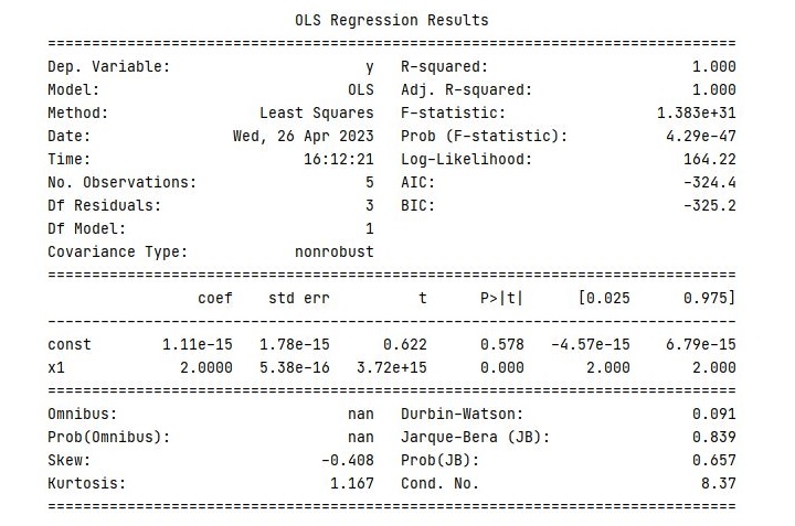
In Python, we can perform inferential statistics using libraries such as Scikit-Learn and StatsModels. Below is an example −

import statsmodels.api as sm
import numpy as np

X = np.array([1,2,3,4,5])
y = np.array([2,4,6,8,10])

X = sm.add_constant(X)
model = sm.OLS(y, X).fit()print(model.summary())

Output

This will output a summary of the regression model, including the coefficients, standard errors, t-statistics, and p-values as follows −

In the next chapter, we will discuss various descriptive and inferential statistics measures, which are commonly used in machine learning, in detail along with Python implementation example.