Category: Machine Learning Miscellaneous

Grid Search is a hyperparameter tuning technique in Machine Learning that helps to find the best combination of hyperparameters for a given model. It works by defining a grid of hyperparameters and then training the model with all the possible combinations of hyperparameters to find the best performing set.

In other words, Grid Search is an exhaustive search method where a set of hyperparameters are defined, and a search is performed over all possible combinations of these hyperparameters to find the optimal values that give the best performance.

Implementation in Python

In Python, Grid Search can be implemented using the GridSearchCV class from the sklearn module. The GridSearchCV class takes the model, the hyperparameters to tune, and a scoring function as input. It then performs an exhaustive search over all possible combinations of hyperparameters and returns the best set of hyperparameters that give the best score.

Here is an example implementation of Grid Search in Python using the GridSearchCV class −

Example

from sklearn.model_selection import GridSearchCV
from sklearn.ensemble import RandomForestClassifier
from sklearn.datasets import make_classification

# Generate a sample dataset
X, y = make_classification(n_samples=1000, n_features=10, n_classes=2)# Define the model and the hyperparameters to tune
model = RandomForestClassifier()
hyperparameters ={'n_estimators':[10,50,100],'max_depth':[None,5,10]}# Define the Grid Search object and fit the data
grid_search = GridSearchCV(model, hyperparameters, scoring='accuracy', cv=5)
grid_search.fit(X, y)# Print the best hyperparameters and the corresponding scoreprint("Best hyperparameters: ", grid_search.best_params_)print("Best score: ", grid_search.best_score_)

In this example, we define a RandomForestClassifier model and a set of hyperparameters to tune, namely the number of trees (n_estimators) and the maximum depth of each tree (max_depth). We then create a GridSearchCV object and fit the data using the fit() method. Finally, we print the best set of hyperparameters and the corresponding score.

Output

When you execute this code, it will produce the following output −

Best hyperparameters: {'max_depth': None, 'n_estimators': 10}
Best score: 0.953

The AUC-ROC curve is a commonly used performance metric in machine learning that is used to evaluate the performance of binary classification models. It is a plot of the true positive rate (TPR) against the false positive rate (FPR) at different threshold values.

What is the AUC-ROC Curve?

The AUC-ROC curve is a graphical representation of the performance of a binary classification model at different threshold values. It plots the true positive rate (TPR) on the y-axis and the false positive rate (FPR) on the x-axis. The TPR is the proportion of actual positive cases that are correctly identified by the model, while the FPR is the proportion of actual negative cases that are incorrectly classified as positive by the model.

The AUC-ROC curve is a useful metric for evaluating the overall performance of a binary classification model because it takes into account the trade-off between TPR and FPR at different threshold values. The area under the curve (AUC) represents the overall performance of the model across all possible threshold values. A perfect classifier would have an AUC of 1.0, while a random classifier would have an AUC of 0.5.

Why is the AUC-ROC Curve Important?

The AUC-ROC curve is an important performance metric in machine learning because it provides a comprehensive measure of a model’s ability to distinguish between positive and negative cases.

It is particularly useful when the data is imbalanced, meaning that one class is much more prevalent than the other. In such cases, accuracy alone may not be a good measure of the model’s performance because it can be skewed by the prevalence of the majority class.

The AUC-ROC curve provides a more balanced view of the model’s performance by taking into account both TPR and FPR.

Implementing the AUC ROC Curve in Python

Now that we understand what the AUC-ROC curve is and why it is important, let’s see how we can implement it in Python. We will use the Scikit-learn library to build a binary classification model and plot the AUC-ROC curve.

First, we need to import the necessary libraries and load the dataset. In this example, we will be using the breast cancer dataset from scikit-learn.

Example

import numpy as np
import pandas as pd
from sklearn.datasets import load_breast_cancer
from sklearn.model_selection import train_test_split
from sklearn.linear_model import LogisticRegression
from sklearn.metrics import roc_auc_score, roc_curve
import matplotlib.pyplot as plt

# load the dataset
data = load_breast_cancer()
X = data.data
y = data.target

# split the data into train and test sets
X_train, X_test, y_train, y_test = train_test_split(X, y, test_size=0.2, random_state=42)

Next, we will fit a logistic regression model to the training set and make predictions on the test set.

# fit a logistic regression model
lr = LogisticRegression()
lr.fit(X_train, y_train)# make predictions on the test set
y_pred = lr.predict_proba(X_test)[:,1]

After making predictions, we can calculate the AUC-ROC score using the roc_auc_score() function from scikit-learn.

# calculate the AUC-ROC score
auc_roc = roc_auc_score(y_test, y_pred)print("AUC-ROC Score:", auc_roc)

This will output the AUC-ROC score for the logistic regression model.

Finally, we can plot the ROC curve using the roc_curve() function and matplotlib library.

# plot the ROC curve
fpr, tpr, thresholds = roc_curve(y_test, y_pred)
plt.plot(fpr, tpr)
plt.title('ROC Curve')
plt.xlabel('False Positive Rate')
plt.ylabel('True Positive Rate')
plt.show()

Output

When you execute this code, it will plot the ROC curve for the logistic regression model.

In addition, it will print the AUC-ROC score on the terminal −

AUC-ROC Score: 0.9967245332459875

Cross-validation is a powerful technique used in machine learning to estimate the performance of a model on unseen data. It is an essential step in building a robust machine learning model, as it helps to identify overfitting or underfitting, and helps to determine the optimal model hyperparameters.

What is Cross-Validation?

Cross-validation is a technique used to evaluate the performance of a model by partitioning the dataset into subsets, training the model on a portion of the data, and then validating the model on the remaining data. The basic idea behind cross-validation is to use a subset of the data to train the model and another subset to test its performance. This allows the machine learning model to be trained on a variety of data and to generalize better to new data.

There are different types of cross-validation techniques available, but the most commonly used technique is k-fold cross-validation. In k-fold cross-validation, the data is partitioned into k equally sized folds. The model is then trained on k-1 folds and tested on the remaining fold. This process is repeated k times, with each of the k folds used once as the validation data. The final performance of the model is then averaged over the k iterations to obtain an estimate of the model’s performance.

Why is Cross-Validation Important?

Cross-validation is an essential technique in machine learning because it helps to prevent overfitting or underfitting of a model. Overfitting occurs when the model is too complex and fits the training data too closely, resulting in poor performance on new data. On the other hand, underfitting occurs when the model is too simple and does not capture the underlying patterns in the data, resulting in poor performance on both the training and test data.

Cross-validation also helps to determine the optimal model hyperparameters. Hyperparameters are the settings that control the behavior of the model. For example, in a decision tree algorithm, the maximum depth of the tree is a hyperparameter that determines the level of complexity of the model. By using cross-validation to evaluate the performance of the model at different hyperparameter values, we can select the optimal hyperparameters that maximize the model’s performance.

Implementing Cross-Validation in Python

In this section, we will discuss how to implement k-fold cross-validation in Python using the Scikit-learn library. Scikit-learn is a popular Python library for machine learning that provides a range of algorithms and tools for data preprocessing, model selection, and evaluation.

To demonstrate how to implement cross-validation in Python, we will use the famous Iris dataset. The Iris dataset contains measurements of the sepal length, sepal width, petal length, and petal width of three different species of iris flowers. The goal is to build a model that can predict the species of an iris flower based on its measurements.

First, we need to load the dataset using the Scikit-learn load_iris() function and split it into a training set and a test set using the train_test_split() function. The training set will be used to train the model, and the test set will be used to evaluate the performance of the model.

from sklearn.datasets import load_iris
from sklearn.model_selection import train_test_split

# Load the Iris dataset
iris = load_iris()# Split the data into a training set and a test set
X_train, X_test, y_train, y_test = train_test_split(iris.data, iris.target, test_size=0.2, random_state=42)

Next, we will create a decision tree classifier using the Scikit-learn DecisionTreeClassifier() function.

from sklearn.tree import DecisionTree

Create a decision tree classifier.

clf = DecisionTreeClassifier(random_state=42)

Now, we can use k-fold cross-validation to evaluate the performance of the model. We will use the cross_val_score() function from Scikit-learn to perform k-fold cross-validation. The function takes as input the model, the training data, the target variable, and the number of folds. It returns an array of scores, one for each fold.

from sklearn.model_selection import cross_val_score

# Perform k-fold cross-validation
scores = cross_val_score(clf, X_train, y_train, cv=5)

Here, we have specified the number of folds as 5, meaning that the data will be partitioned into 5 equally sized folds. The cross_val_score() function will train the model on 4 folds and test it on the remaining fold. This process will be repeated 5 times, with each fold used once as the validation data. The function returns an array of scores, one for each fold.

Finally, we can calculate the mean and standard deviation of the scores to get an estimate of the model’s performance.

import numpy as np

# Calculate the mean and standard deviation of the scores
mean_score = np.mean(scores)
std_score = np.std(scores)print("Mean cross-validation score: {:.2f}".format(mean_score))print("Standard deviation of cross-validation score: {:.2f}".format(std_score))

The output of this code will be the mean and standard deviation of the scores. The mean score represents the average performance of the model across all folds, while the standard deviation represents the variability of the scores.

Example

Here is the complete implementation of Cross-Validation in Python −

from sklearn.datasets import load_iris
from sklearn.tree import DecisionTreeClassifier
from sklearn.model_selection import cross_val_score
import numpy as np

# Load the iris dataset
iris = load_iris()# Define the features and target variables
X = iris.data
y = iris.target

# Create a decision tree classifier
clf = DecisionTreeClassifier(random_state=42)# Perform k-fold cross-validation
scores = cross_val_score(clf, X, y, cv=5)# Calculate the mean and standard deviation of the scores
mean_score = np.mean(scores)
std_score = np.std(scores)print("Mean cross-validation score: {:.2f}".format(mean_score))print("Standard deviation of cross-validation score: {:.2f}".format(std_score))

Output

When you execute this code, it will produce the following output −

Mean cross-validation score: 0.95
Standard deviation of cross-validation score: 0.03

Bagging is an ensemble learning technique that combines the predictions of multiple models to improve the accuracy and stability of a single model. It involves creating multiple subsets of the training data by randomly sampling with replacement. Each subset is then used to train a separate model, and the final prediction is made by averaging the predictions of all models.

The main idea behind Bagging is to reduce the variance of a single model by using multiple models that are less complex but still accurate. By averaging the predictions of multiple models, Bagging reduces the risk of overfitting and improves the stability of the model.

How Does Bagging Work?

The Bagging algorithm works in the following steps −

• Create multiple subsets of the training data by randomly sampling with replacement.
• Train a separate model on each subset of the data.
• Make predictions on the testing data using each model.
• Combine the predictions of all models by taking the average or majority vote.

The key feature of Bagging is that each model is trained on a different subset of the training data, which introduces diversity into the ensemble. The models are typically trained using a base model, such as a decision tree, logistic regression, or support vector machine.

Example

Now let’s see how we can implement Bagging in Python using the Scikit-learn library. For this example, we will use the famous Iris dataset.

from sklearn.datasets import load_iris
from sklearn.ensemble import BaggingClassifier
from sklearn.tree import DecisionTreeClassifier
from sklearn.model_selection import train_test_split
from sklearn.metrics import accuracy_score

# Load the Iris dataset
iris = load_iris()# Split the data into training and testing sets
X_train, X_test, y_train, y_test = train_test_split(iris.data, iris.target, test_size=0.2, random_state=42)# Define the base estimator
base_estimator = DecisionTreeClassifier(max_depth=3)# Define the Bagging classifier
bagging = BaggingClassifier(base_estimator=base_estimator, n_estimators=10, random_state=42)# Train the Bagging classifier
bagging.fit(X_train, y_train)# Make predictions on the testing set
y_pred = bagging.predict(X_test)# Evaluate the model's accuracy
accuracy = accuracy_score(y_test, y_pred)print("Accuracy:", accuracy)

In this example, we first load the Iris dataset using Scikit-learn’s load_iris function and split it into training and testing sets using the train_test_split function.

We then define the base estimator, which is a decision tree with a maximum depth of 3, and the Bagging classifier, which consists of 10 decision trees.

We train the Bagging classifier using the fit method and make predictions on the testing set using the predict method. Finally, we evaluate the model’s accuracy using the accuracy_score function from Scikit-learn’s metrics module.

Output

When you execute this code, it will produce the following output −

Accuracy: 1.0

Gradient Boosting Machines (GBM) is a powerful machine learning technique that is widely used for building predictive models. It is a type of ensemble method that combines the predictions of multiple weaker models to create a stronger and more accurate model.

GBM is a popular choice for a wide range of applications, including regression, classification, and ranking problems. Let’s understand the workings of GBM and how it can be used in machine learning.

What is a Gradient Boosting Machine (GBM)?

GBM is an iterative machine learning algorithm that combines the predictions of multiple decision trees to make a final prediction.

The algorithm works by training a sequence of decision trees, each of which is designed to correct the errors of the previous tree.

In each iteration, the algorithm identifies the samples in the dataset that are most difficult to predict and focuses on improving the model’s performance on these samples.

This is achieved by fitting a new decision tree that is optimized to reduce the errors on the difficult samples. The process continues until a specified stopping criteria is met, such as reaching a certain level of accuracy or the maximum number of iterations.

How Does a Gradient Boosting Machine Work?

The basic steps involved in training a GBM model are as follows −

• Initialize the model − The algorithm starts by creating a simple model, such as a single decision tree, to serve as the initial model.
• Calculate residuals − The initial model is used to make predictions on the training data, and the residuals are calculated as the differences between the predicted values and the actual values.
• Train a new model − A new decision tree is trained on the residuals, with the goal of minimizing the errors on the difficult samples.
• Update the model − The predictions of the new model are added to the predictions of the previous model, and the residuals are recalculated based on the updated predictions.
• Repeat − Steps 3-4 are repeated until a specified stopping criteria is met.

GBM can be further improved by introducing regularization techniques, such as L1 and L2 regularization, to prevent overfitting. Additionally, GBM can be extended to handle categorical variables, missing data, and multi-class classification problems.

Example

Here is an example of implementing GBM using the Sklearn breast cancer dataset −

from sklearn.datasets import load_breast_cancer
from sklearn.model_selection import train_test_split
from sklearn.ensemble import GradientBoostingClassifier
from sklearn.metrics import accuracy_score

# Load the breast cancer dataset
data = load_breast_cancer()
X = data.data
y = data.target

# Split the data into training and testing sets
X_train, X_test, y_train, y_test = train_test_split(X, y, test_size=0.2, random_state=42)# Train the model using GradientBoostingClassifier
model = GradientBoostingClassifier(n_estimators=100, max_depth=3, learning_rate=0.1)
model.fit(X_train, y_train)# Make predictions on the testing set
y_pred = model.predict(X_test)# Evaluate the model's accuracy
accuracy = accuracy_score(y_test, y_pred)print("Accuracy:", accuracy)

Output

In this example, we load the breast cancer dataset using Sklearn’s load_breast_cancer function and split it into training and testing sets. We then define the parameters for the GBM model using GradientBoostingClassifier, including the number of estimators (i.e., the number of decision trees), the maximum depth of each decision tree, and the learning rate.

We train the GBM model using the fit method and make predictions on the testing set using the predict method. Finally, we evaluate the model’s accuracy using the accuracy_score function from Sklearn’s metrics module.

When you execute this code, it will produce the following output −

Accuracy: 0.956140350877193

Advantages of Using Gradient Boosting Machines

There are several advantages of using GBM in machine learning −

• High accuracy − GBM is known for its high accuracy, as it combines the predictions of multiple weaker models to create a stronger and more accurate model.
• Robustness − GBM is robust to outliers and noisy data, as it focuses on improving the model’s performance on the most difficult samples.
• Flexibility − GBM can be used for a wide range of applications, including regression, classification, and ranking problems.
• Interpretability − GBM provides insights into the importance of different features in making predictions, which can be useful for understanding the underlying factors driving the predictions.
• Scalability − GBM can handle large datasets and can be parallelized to accelerate the training process.

Limitations of Gradient Boosting Machines

There are also some limitations to using GBM in machine learning −

• Training time − GBM can be computationally expensive and may require a significant amount of training time, especially when working with large datasets.
• Hyperparameter tuning − GBM requires careful tuning of hyperparameters, such as the learning rate, number of trees, and maximum depth, to achieve optimal performance.
• Black box model − GBM can be difficult to interpret, as the final model is a combination of multiple decision trees and may not provide clear insights into the underlying factors driving the predictions.

Boosting is a popular ensemble learning technique that combines several weak learners to create a strong learner. It works by iteratively training weak learners on subsets of the data and assigning higher weights to the misclassified samples to increase their importance in the subsequent iterations. This process is repeated until the desired level of performance is achieved.

Here are some techniques to boost model performance in machine learning −

• Feature Engineering − Feature engineering involves creating new features from the existing features or transforming the existing features to make them more informative for the model. This can include techniques such as one-hot encoding, scaling, normalization, and feature selection.
• Hyperparameter Tuning − Hyperparameters are parameters that are not learned during training but are set by the data scientist. They control the behavior of the model, and tuning them can significantly impact model performance. Grid search and randomized search are common techniques for hyperparameter tuning.
• Ensemble Learning − Ensemble learning involves combining multiple models to improve performance. Techniques such as bagging, boosting, and stacking can be used to create ensembles. Random forests are an example of a bagging ensemble, while gradient boosting machines (GBMs) are an example of a boosting ensemble.
• Regularization − Regularization is a technique that prevents overfitting by adding a penalty term to the loss function. L1 regularization (Lasso) and L2 regularization (Ridge) are common techniques used in linear models, while dropout is a technique used in neural networks.
• Data Augmentation − Data augmentation involves generating new data from the existing data by applying transformations such as rotation, scaling, and flipping. This can help to reduce overfitting and improve model performance.
• Model Architecture − The architecture of the model can significantly impact its performance. Techniques such as deep learning and convolutional neural networks (CNNs) can be used to create more complex models that are better able to learn complex patterns in the data.
• Early Stopping − Early stopping is a technique used to prevent overfitting by stopping the training process once the model performance stops improving on a validation set. This prevents the model from continuing to learn the noise in the data and can help to improve generalization.
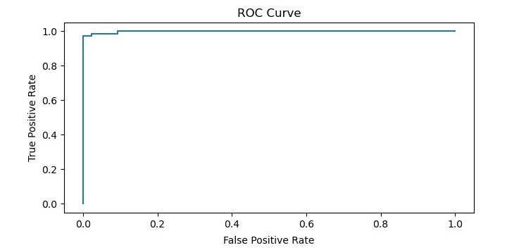
• Cross-Validation − Cross-validation is a technique used to evaluate the performance of a model on multiple subsets of the data. This can help to identify overfitting and can be used to select the best hyperparameters for the model.

These techniques can be implemented in Python using various machine learning libraries such as scikit-learn, TensorFlow, and Keras. By using these techniques, data scientists can improve the performance of their models and create more accurate predictions.

The following example below in which implement cross-validation using Scikit-learn −

Example

from sklearn.datasets import load_iris
from sklearn.model_selection import cross_val_score
from sklearn.ensemble import GradientBoostingClassifier

# Load the iris dataset
iris = load_iris()
X = iris.data
y = iris.target

# Create a Gradient Boosting Classifier
gb_clf = GradientBoostingClassifier()# Perform 5-fold cross-validation on the classifier
scores = cross_val_score(gb_clf, X, y, cv=5)# Print the average accuracy and standard deviation of the cross-validation scoresprint("Accuracy: %0.2f (+/- %0.2f)"%(scores.mean(), scores.std()*2))

Output

When you execute this code, it will produce the following output −

Accuracy: 0.96 (+/- 0.07)

Performance Improvement with Ensembles

Ensembles can give us boost in the machine learning result by combining several models. Basically, ensemble models consist of several individually trained supervised learning models and their results are merged in various ways to achieve better predictive performance compared to a single model. Ensemble methods can be divided into following two groups −

Sequential ensemble methods

As the name implies, in these kind of ensemble methods, the base learners are generated sequentially. The motivation of such methods is to exploit the dependency among base learners.

Parallel ensemble methods

As the name implies, in these kind of ensemble methods, the base learners are generated in parallel. The motivation of such methods is to exploit the independence among base learners.

Ensemble Learning Methods

The following are the most popular ensemble learning methods i.e. the methods for combining the predictions from different models −

Bagging

The term bagging is also known as bootstrap aggregation. In bagging methods, ensemble model tries to improve prediction accuracy and decrease model variance by combining predictions of individual models trained over randomly generated training samples. The final prediction of ensemble model will be given by calculating the average of all predictions from the individual estimators. One of the best examples of bagging methods are random forests.

Boosting

In boosting method, the main principle of building ensemble model is to build it incrementally by training each base model estimator sequentially. As the name suggests, it basically combine several week base learners, trained sequentially over multiple iterations of training data, to build powerful ensemble. During the training of week base learners, higher weights are assigned to those learners which were misclassified earlier. The example of boosting method is AdaBoost.

Voting

In this ensemble learning model, multiple models of different types are built and some simple statistics, like calculating mean or median etc., are used to combine the predictions. This prediction will serve as the additional input for training to make the final prediction.

Bagging Ensemble Algorithms

The following are three bagging ensemble algorithms −

Bagged Decision Tree

As we know that bagging ensemble methods work well with the algorithms that have high variance and, in this concern, the best one is decision tree algorithm. In the following Python recipe, we are going to build bagged decision tree ensemble model by using BaggingClassifier function of sklearn with DecisionTreeClasifier (a classification & regression trees algorithm) on Pima Indians diabetes dataset.

First, import the required packages as follows −

from pandas import read_csv
from sklearn.model_selection import KFold
from sklearn.model_selection import cross_val_score
from sklearn.ensemble import BaggingClassifier
from sklearn.tree import DecisionTreeClassifier

Now, we need to load the Pima diabetes dataset as we did in the previous examples −

path =r"C:\pima-indians-diabetes.csv"
headernames =['preg','plas','pres','skin','test','mass','pedi','age','class']
data = read_csv(path, names=headernames)
array = data.values
X = array[:,0:8]
Y = array[:,8]

Next, give the input for 10-fold cross validation as follows −

seed =7
kfold = KFold(n_splits=10, random_state=seed)
cart = DecisionTreeClassifier()

We need to provide the number of trees we are going to build. Here we are building 150 trees −

num_trees =150

Next, build the model with the help of following script −

model = BaggingClassifier(base_estimator=cart, n_estimators=num_trees, random_state=seed)

Calculate and print the result as follows −

results = cross_val_score(model, X, Y, cv=kfold)print(results.mean())

Output

0.7733766233766234

The output above shows that we got around 77% accuracy of our bagged decision tree classifier model.

Random Forest

It is an extension of bagged decision trees. For individual classifiers, the samples of training dataset are taken with replacement, but the trees are constructed in such a way that reduces the correlation between them. Also, a random subset of features is considered to choose each split point rather than greedily choosing the best split point in construction of each tree.

In the following Python recipe, we are going to build bagged random forest ensemble model by using RandomForestClassifier class of sklearn on Pima Indians diabetes dataset.

First, import the required packages as follows −

from pandas import read_csv
from sklearn.model_selection import KFold
from sklearn.model_selection import cross_val_score
from sklearn.ensemble import RandomForestClassifier

Now, we need to load the Pima diabetes dataset as did in previous examples −

path =r"C:\pima-indians-diabetes.csv"
headernames =['preg','plas','pres','skin','test','mass','pedi','age','class']
data = read_csv(path, names=headernames)
array = data.values
X = array[:,0:8]
Y = array[:,8]

Next, give the input for 10-fold cross validation as follows −

seed =7
kfold = KFold(n_splits=10, random_state=seed)

We need to provide the number of trees we are going to build. Here we are building 150 trees with split points chosen from 5 features −

num_trees =150
max_features =5

Next, build the model with the help of following script −

model = RandomForestClassifier(n_estimators=num_trees, max_features=max_features)

Calculate and print the result as follows −

results = cross_val_score(model, X, Y, cv=kfold)print(results.mean())

Output

0.7629357484620642

The output above shows that we got around 76% accuracy of our bagged random forest classifier model.

Extra Trees

It is another extension of bagged decision tree ensemble method. In this method, the random trees are constructed from the samples of the training dataset.

In the following Python recipe, we are going to build extra tree ensemble model by using ExtraTreesClassifier class of sklearn on Pima Indians diabetes dataset.

First, import the required packages as follows −

from pandas import read_csv
from sklearn.model_selection import KFold
from sklearn.model_selection import cross_val_score
from sklearn.ensemble import ExtraTreesClassifier

Now, we need to load the Pima diabetes dataset as did in previous examples −

path =r"C:\pima-indians-diabetes.csv"
headernames =['preg','plas','pres','skin','test','mass','pedi','age','class']
data = read_csv(path, names=headernames)
array = data.values
X = array[:,0:8]
Y = array[:,8]

Next, give the input for 10-fold cross validation as follows −

seed =7
kfold = KFold(n_splits=10, random_state=seed)

We need to provide the number of trees we are going to build. Here we are building 150 trees with split points chosen from 5 features −

num_trees =150
max_features =5

Next, build the model with the help of following script −

model = ExtraTreesClassifier(n_estimators=num_trees, max_features=max_features)

Calculate and print the result as follows −

results = cross_val_score(model, X, Y, cv=kfold)print(results.mean())

Output

0.7551435406698566

The output above shows that we got around 75.5% accuracy of our bagged extra trees classifier model.

Boosting Ensemble Algorithms

The followings are the two most common boosting ensemble algorithms −

AdaBoost

It is one the most successful boosting ensemble algorithm. The main key of this algorithm is in the way they give weights to the instances in dataset. Due to this the algorithm needs to pay less attention to the instances while constructing subsequent models.

In the following Python recipe, we are going to build Ada Boost ensemble model for classification by using AdaBoostClassifier class of sklearn on Pima Indians diabetes dataset.

First, import the required packages as follows −

from pandas import read_csv
from sklearn.model_selection import KFold
from sklearn.model_selection import cross_val_score
from sklearn.ensemble import AdaBoostClassifier

Now, we need to load the Pima diabetes dataset as did in previous examples −

path =r"C:\pima-indians-diabetes.csv"
headernames =['preg','plas','pres','skin','test','mass','pedi','age','class']
data = read_csv(path, names=headernames)
array = data.values
X = array[:,0:8]
Y = array[:,8]

Next, give the input for 10-fold cross validation as follows −

seed =5
kfold = KFold(n_splits=10, random_state=seed)

We need to provide the number of trees we are going to build. Here we are building 150 trees with split points chosen from 5 features −

num_trees =50

Next, build the model with the help of following script −

model = AdaBoostClassifier(n_estimators=num_trees, random_state=seed)

Calculate and print the result as follows −

results = cross_val_score(model, X, Y, cv=kfold)print(results.mean())

Output

0.7539473684210527

The output above shows that we got around 75% accuracy of our AdaBoost classifier ensemble model.

Stochastic Gradient Boosting

It is also called Gradient Boosting Machines. In the following Python recipe, we are going to build Stochastic Gradient Boostingensemble model for classification by using GradientBoostingClassifier class of sklearn on Pima Indians diabetes dataset.

First, import the required packages as follows −

from pandas import read_csv
from sklearn.model_selection import KFold
from sklearn.model_selection import cross_val_score
from sklearn.ensemble import GradientBoostingClassifier

Now, we need to load the Pima diabetes dataset as did in previous examples −

path =r"C:\pima-indians-diabetes.csv"
headernames =['preg','plas','pres','skin','test','mass','pedi','age','class']
data = read_csv(path, names=headernames)
array = data.values
X = array[:,0:8]
Y = array[:,8]

Next, give the input for 10-fold cross validation as follows −

seed =5
kfold = KFold(n_splits=10, random_state=seed)

We need to provide the number of trees we are going to build. Here we are building 150 trees with split points chosen from 5 features −

num_trees =50

Next, build the model with the help of following script −

model = GradientBoostingClassifier(n_estimators=num_trees, random_state=seed)

Calculate and print the result as follows −

results = cross_val_score(model, X, Y, cv=kfold)print(results.mean())

Output

0.7746582365003418

The output above shows that we got around 77.5% accuracy of our Gradient Boosting classifier ensemble model.

Voting Ensemble Algorithms

As discussed, voting first creates two or more standalone models from training dataset and then a voting classifier will wrap the model along with taking the average of the predictions of sub-model whenever needed new data.

In the following Python recipe, we are going to build Voting ensemble model for classification by using VotingClassifier class of sklearn on Pima Indians diabetes dataset. We are combining the predictions of logistic regression, Decision Tree classifier and SVM together for a classification problem as follows −

First, import the required packages as follows −

from pandas import read_csv
from sklearn.model_selection import KFold
from sklearn.model_selection import cross_val_score
from sklearn.linear_model import LogisticRegression
from sklearn.tree import DecisionTreeClassifier
from sklearn.svm import SVC
from sklearn.ensemble import VotingClassifier

Now, we need to load the Pima diabetes dataset as did in previous examples −

path =r"C:\pima-indians-diabetes.csv"
headernames =['preg','plas','pres','skin','test','mass','pedi','age','class']
data = read_csv(path, names=headernames)
array = data.values
X = array[:,0:8]
Y = array[:,8]

Next, give the input for 10-fold cross validation as follows −

kfold = KFold(n_splits=10, random_state=7)

Next, we need to create sub-models as follows −

estimators =[]
model1 = LogisticRegression()
estimators.append(('logistic', model1))
model2 = DecisionTreeClassifier()
estimators.append(('cart', model2))
model3 = SVC()
estimators.append(('svm', model3))

Now, create the voting ensemble model by combining the predictions of above created sub models.

ensemble = VotingClassifier(estimators)
results = cross_val_score(ensemble, X, Y, cv=kfold)print(results.mean())

Output

0.7382262474367738

The output above shows that we got around 74% accuracy of our voting classifier ensemble model.

Introduction

In order to execute and produce results successfully, a machine learning model must automate some standard workflows. The process of automate these standard workflows can be done with the help of Scikit-learn Pipelines. From a data scientists perspective, pipeline is a generalized, but very important concept. It basically allows data flow from its raw format to some useful information. The working of pipelines can be understood with the help of following diagram −

The blocks of ML pipelines are as follows −

Data ingestion − As the name suggests, it is the process of importing the data for use in ML project. The data can be extracted in real time or batches from single or multiple systems. It is one of the most challenging steps because the quality of data can affect the whole ML model.

Data Preparation − After importing the data, we need to prepare data to be used for our ML model. Data preprocessing is one of the most important technique of data preparation.

ML Model Training − Next step is to train our ML model. We have various ML algorithms like supervised, unsupervised, reinforcement to extract the features from data, and make predictions.

Model Evaluation − Next, we need to evaluate the ML model. In case of AutoML pipeline, ML model can be evaluated with the help of various statistical methods and business rules.

ML Model retraining − In case of AutoML pipeline, it is not necessary that the first model is best one. The first model is considered as a baseline model and we can train it repeatably to increase models accuracy.

Deployment − At last, we need to deploy the model. This step involves applying and migrating the model to business operations for their use.

Challenges Accompanying ML Pipelines

In order to create ML pipelines, data scientists face many challenges. These challenges fall into the following three categories −

Quality of Data

The success of any ML model depends heavily on the quality of data. If the data we are providing to ML model is not accurate, reliable and robust, then we are going to end with wrong or misleading output.

Data Reliability

Another challenge associated with ML pipelines is the reliability of data we are providing to the ML model. As we know, there can be various sources from which data scientist can acquire data but to get the best results, it must be assured that the data sources are reliable and trusted.

Data Accessibility

To get the best results out of ML pipelines, the data itself must be accessible which requires consolidation, cleansing and curation of data. As a result of data accessibility property, metadata will be updated with new tags.

Modelling ML Pipeline and Data Preparation

Data leakage, happening from training dataset to testing dataset, is an important issue for data scientist to deal with while preparing data for ML model. Generally, at the time of data preparation, data scientist uses techniques like standardization or normalization on entire dataset before learning. But these techniques cannot help us from the leakage of data because the training dataset would have been influenced by the scale of the data in the testing dataset.

By using ML pipelines, we can prevent this data leakage because pipelines ensure that data preparation like standardization is constrained to each fold of our cross-validation procedure.

Example

The following is an example in Python that demonstrate data preparation and model evaluation workflow. For this purpose, we are using Pima Indian Diabetes dataset from Sklearn. First, we will be creating pipeline that standardized the data. Then a Linear Discriminative analysis model will be created and at last the pipeline will be evaluated using 10-fold cross validation.

First, import the required packages as follows −

from pandas import read_csv
from sklearn.model_selection import KFold
from sklearn.model_selection import cross_val_score
from sklearn.preprocessing import StandardScaler
from sklearn.pipeline import Pipeline
from sklearn.discriminant_analysis import LinearDiscriminantAnalysis

Now, we need to load the Pima diabetes dataset as did in previous examples −

path =r"C:\pima-indians-diabetes.csv"
headernames =['preg','plas','pres','skin','test','mass','pedi','age','class']
data = read_csv(path, names=headernames)
array = data.values

Next, we will create a pipeline with the help of the following code −

estimators =[]
estimators.append(('standardize', StandardScaler()))
estimators.append(('lda', LinearDiscriminantAnalysis()))
model = Pipeline(estimators)

At last, we are going to evaluate this pipeline and output its accuracy as follows −

kfold = KFold(n_splits=20, random_state=7)
results = cross_val_score(model, X, Y, cv=kfold)print(results.mean())

Output

0.7790148448043184

The above output is the summary of accuracy of the setup on the dataset.

Modelling ML Pipeline and Feature Extraction

Data leakage can also happen at feature extraction step of ML model. That is why feature extraction procedures should also be restricted to stop data leakage in our training dataset. As in the case of data preparation, by using ML pipelines, we can prevent this data leakage also. FeatureUnion, a tool provided by ML pipelines can be used for this purpose.

Example

The following is an example in Python that demonstrates feature extraction and model evaluation workflow. For this purpose, we are using Pima Indian Diabetes dataset from Sklearn.

First, 3 features will be extracted with PCA (Principal Component Analysis). Then, 6 features will be extracted with Statistical Analysis. After feature extraction, result of multiple feature selection and extraction procedures will be combined by using

FeatureUnion tool. At last, a Logistic Regression model will be created, and the pipeline will be evaluated using 10-fold cross validation.

First, import the required packages as follows −

from pandas import read_csv
from sklearn.model_selection import KFold
from sklearn.model_selection import cross_val_score
from sklearn.pipeline import Pipeline
from sklearn.pipeline import FeatureUnion
from sklearn.linear_model import LogisticRegression
from sklearn.decomposition import PCA
from sklearn.feature_selection import SelectKBest

Now, we need to load the Pima diabetes dataset as did in previous examples −

path =r"C:\pima-indians-diabetes.csv"
headernames =['preg','plas','pres','skin','test','mass','pedi','age','class']
data = read_csv(path, names=headernames)
array = data.values

Next, feature union will be created as follows −

features =[]
features.append(('pca', PCA(n_components=3)))
features.append(('select_best', SelectKBest(k=6)))
feature_union = FeatureUnion(features)

Next, pipeline will be creating with the help of following script lines −

estimators =[]
estimators.append(('feature_union', feature_union))
estimators.append(('logistic', LogisticRegression()))
model = Pipeline(estimators)

At last, we are going to evaluate this pipeline and output its accuracy as follows −

kfold = KFold(n_splits=20, random_state=7)
results = cross_val_score(model, X, Y, cv=kfold)print(results.mean())

Output

0.7789811066126855

Performance Metrics in Machine Learning

Performance metrics in machine learning are used to evaluate the performance of a machine learning model. These metrics provide quantitative measures to assess how well a model is performing and to compare the performance of different models. Performance metrics are important because they help us understand how well our model is performing and whether it is meeting our requirements. In this way, we can make informed decisions about whether to use a particular model or not.

We must carefully choose the metrics for evaluating ML performance because −

• How the performance of ML algorithms is measured and compared will be dependent entirely on the metric you choose.
• How you weight the importance of various characteristics in the result will be influenced completely by the metric you choose.

There are various metrics which we can use to evaluate the performance of ML algorithms, classification as well as regression algorithms. Let’s discuss these metrics for Classification and Regression problems separately.

Performance Metrics for Classification Problems

We have discussed classification and its algorithms in the previous chapters. Here, we are going to discuss various performance metrics that can be used to evaluate predictions for classification problems.

• Confusion Matrix
• Classification Accuracy
• Classification Report
• Precision
• Recall or Sensitivity
• Specificity
• Support
• F1 Score
• ROC AUC Score
• LOGLOSS (Logarithmic Loss)

Confusion Matrix

The consfusion matrix is the easiest way to measure the performance of a classification problem where the output can be of two or more type of classes. A confusion matrix is nothing but a table with two dimensions viz. “Actual” and “Predicted” and furthermore, both the dimensions have “True Positives (TP)”, “True Negatives (TN)”, “False Positives (FP)”, “False Negatives (FN)” as shown below −

Explanation of the terms associated with confusion matrix are as follows −

• True Positives (TP) − It is the case when both actual class & predicted class of data point is 1.
• True Negatives (TN) − It is the case when both actual class & predicted class of data point is 0.
• False Positives (FP) − It is the case when actual class of data point is 0 & predicted class of data point is 1.
• False Negatives (FN) − It is the case when actual class of data point is 1 & predicted class of data point is 0.

We can use confusion_matrix function of sklearn.metrics to compute Confusion Matrix of our classification model.

Classification Accuracy

Accuracy is most common performance metric for classification algorithms. It may be defined as the number of correct predictions made as a ratio of all predictions made. We can easily calculate it by confusion matrix with the help of following formula −

Accuracy=TP+TN𝑇𝑃+𝐹𝑃+𝐹𝑁+𝑇𝑁

We can use accuracy_score function of sklearn.metrics to compute accuracy of our classification model.

Classification Report

This report consists of the scores of Precisions, Recall, F1 and Support. They are explained as follows −

Precision

Precision measures the proportion of true positive instances out of all predicted positive instances. It is calculated as the number of true positive instances divided by the sum of true positive and false positive instances.

We can easily calculate it by confusion matrix with the help of following formula −

Precision=TPTP+FP

Precision, used in document retrievals, may be defined as the number of correct documents returned by our ML model.

Recall or Sensitivity

Recall measures the proportion of true positive instances out of all actual positive instances. It is calculated as the number of true positive instances divided by the sum of true positive and false negative instances.

We can easily calculate it by confusion matrix with the help of following formula −

Recall=TPTP+FN

Specificity

Specificity, in contrast to recall, may be defined as the number of negatives returned by our ML model. We can easily calculate it by confusion matrix with the help of following formula −

Specificity=TNTN+FP

Support

Support may be defined as the number of samples of the true response that lies in each class of target values.

F1 Score

F1 score is the harmonic mean of precision and recall. It is a balanced measure that takes into account both precision and recall. Mathematically, F1 score is the weighted average of the precision and recall. The best value of F1 would be 1 and worst would be 0. We can calculate F1 score with the help of following formula −

F1=2∗(precision∗recall)/(precision+recall))

F1 score is having equal relative contribution of precision and recall.

We can use classification_report function of sklearn.metrics to get the classification report of our classification model.

ROC AUC Score

The ROC (Receiver Operating Characteristic) Area Under the Curve(AUC) score is a measure of the ability of a classifier to distinguish between positive and negative instances. It is calculated by plotting the true positive rate against the false positive rate at different classification thresholds and calculating the area under the curve.

As name suggests, ROC is a probability curve and AUC measure the separability. In simple words, ROC-AUC score will tell us about the capability of model in distinguishing the classes. Higher the score, better the model.

We can use roc_auc_score function of sklearn.metrics to compute AUC-ROC.

LOGLOSS (Logarithmic Loss)

It is also called Logistic regression loss or cross-entropy loss. It basically defined on probability estimates and measures the performance of a classification model where the input is a probability value between 0 and 1. It can be understood more clearly by differentiating it with accuracy. As we know that accuracy is the count of predictions (predicted value = actual value) in our model whereas Log Loss is the amount of uncertainty of our prediction based on how much it varies from the actual label. With the help of Log Loss value, we can have more accurate view of the performance of our model. We can use log_loss function of sklearn.metrics to compute Log Loss.

Example

The following is a simple recipe in Python which will give us an insight about how we can use the above explained performance metrics on binary classification model −

from sklearn.metrics import confusion_matrix
from sklearn.metrics import accuracy_score
from sklearn.metrics import classification_report
from sklearn.metrics import roc_auc_score
from sklearn.metrics import log_loss
X_actual =[1,1,0,1,0,0,1,0,0,0]
Y_predic =[1,0,1,1,1,0,1,1,0,0]
results = confusion_matrix(X_actual, Y_predic)print('Confusion Matrix :')print(results)print('Accuracy Score is',accuracy_score(X_actual, Y_predic))print('Classification Report : ')print(classification_report(X_actual, Y_predic))print('AUC-ROC:',roc_auc_score(X_actual, Y_predic))print('LOGLOSS Value is',log_loss(X_actual, Y_predic))

Output

Confusion Matrix :
[
   [3 3]
   [1 3]
]
Accuracy Score is 0.6
Classification Report :
            precision      recall      f1-score       support
      0       0.75          0.50      0.60           6
      1       0.50          0.75      0.60           4
micro avg     0.60          0.60      0.60           10
macro avg     0.62          0.62      0.60           10
weighted avg  0.65          0.60      0.60           10
AUC-ROC:  0.625
LOGLOSS Value is 13.815750437193334

Performance Metrics for Regression Problems

We have discussed regression and its algorithms in previous chapters. Here, we are going to discuss various performance metrics that can be used to evaluate predictions for regression problems.

• Mean Absolute Error (MAE)
• Mean Square Error (MSE)
• R Squared (R²) Score

Mean Absolute Error (MAE)

It is the simplest error metric used in regression problems. It is basically the sum of average of the absolute difference between the predicted and actual values. In simple words, with MAE, we can get an idea of how wrong the predictions were. MAE does not indicate the direction of the model i.e. no indication about underperformance or overperformance of the model. The following is the formula to calculate MAE −

MAE=1n∑|Y−Ŷ |

Here, 𝑌=Actual Output Values

And Ŷ = Predicted Output Values.

We can use mean_absolute_error function of sklearn.metrics to compute MAE.

Mean Square Error (MSE)

MSE is like the MAE, but the only difference is that the it squares the difference of actual and predicted output values before summing them all instead of using the absolute value. The difference can be noticed in the following equation −

MSE=1n∑(Y−Ŷ )

Here, 𝑌=Actual Output Values

And Ŷ  = Predicted Output Values.

We can use mean_squared_error function of sklearn.metrics to compute MSE.

R Squared (R²) Score

R Squared metric is generally used for explanatory purpose and provides an indication of the goodness or fit of a set of predicted output values to the actual output values. The following formula will help us understanding it −

R2=1−1n∑ni=1(Yi−Yi^)21n∑ni=1(Yi−Yi)2¯

In the above equation, numerator is MSE and the denominator is the variance in 𝑌 values.

We can use r2_score function of sklearn.metrics to compute R squared value.

Example

The following is a simple recipe in Python which will give us an insight about how we can use the above explained performance metrics on regression model −

from sklearn.metrics import r2_score
from sklearn.metrics import mean_absolute_error
from sklearn.metrics import mean_squared_error
X_actual =[5,-1,2,10]
Y_predic =[3.5,-0.9,2,9.9]print('R Squared =',r2_score(X_actual, Y_predic))print('MAE =',mean_absolute_error(X_actual, Y_predic))print('MSE =',mean_squared_error(X_actual, Y_predic))

Output

R Squared = 0.9656060606060606
MAE = 0.42499999999999993
MSE = 0.5674999999999999