Supervised learning and Unsupervised learning are two popular approaches in Machine Learning. The simplest way to distinguish between supervised and unsupervised learning is the type of training dataset and the way the models are trained. However, there are other differences, which are further discussed in the chapter.
What is Supervised Learning?
Supervised Learning is a machine learning approach that uses labeled datasets to train the model, making it ideal for tasks like classifying data or predicting output. Supervised learning is categorized into two types −
1. Classification
Classification uses algorithms to predict categorical values, such as determining whether an email is spam or not or whether it is true or false. The algorithm learns to map each input to its corresponding output label. Some common algorithms include K-Nearest Neighbors, Random forests and Decision trees.
2. Regression
Regression is a statistical approach to analyze the relationship between data points. It can be used to forecast house prices based on features like location and size or estimate future sales. Some common algorithms include linear regression, polynomial regression, and logistic regression.
What is Unsupervised Learning?
Unsupervised Learning is a machine learning approach used to train models on raw and unlabeled data. This approach is often used to identify patterns in the data without human supervision. Unsupervised learning models are used to for the below tasks −
1. Clustering
This task uses unsupervised learning models to group data points into clusters based on their similarities. Popular algorithm used is the K-means clustering.
2. Association
This is another type of unsupervised learning that uses pre-defined rules to group data points into a cluster. It is commonly used in Market Basket Analysis, and the main algorithm behind this task is Apriori Algorithm.
3. Dimensionality Reduction
This method of unsupervised learning is used to reduce the size of a dataset by removing features that are not necessary without compromising the originality of the data.
Differences between Supervised and Unsupervised Learning
The table below shows some key differences between supervised and unsupervised machine learning −
Basis
Supervised Learning
Unsupervised Learning
Definition
Supervised learning algorithms train data, where every input has a corresponding output.
Unsupervised learning algorithms find patterns in data that has no predefined labels.
Goal
The goal of supervised learning is to predict or classify based on input features.
The goal of unsupervised learning is to discover hidden patterns, structures and relationships.
Input Data
Labeled: Input data with corresponding output labels.
Unlabeled: Input data is raw and unlabeled.
Human Supervision
Supervised learning algorithms needs human supervision to train the model.
Unsupervised learning algorithms does not any kind of supervision to train the model..
Tasks
Regression, Classification
Clustering, Association and Dimensionality Reduction
Complexity
supervised machine learning methods are computationally simple.
Unsupervised machine learning methods are computationally complex.
Algorithms
Linear regression, K-Nearest Neighbors, Decision Trees, Naive Bayes, SVM
K- Means clustering, DBSCAN, Autoencoders
Accuracy
Supervised machine learning methods are highly accurate.
Unsupervised machine learning methods are less accurate.
Applications
Image classification, Sentiment Analysis, Recommendation systems
Supervised or Unsupervised Learning – Which to Choose?
Choosing the right approach is crucial and will also determine the efficiency of the outcome. To decide on which learning approach is best, the following things should be considered −
Dataset − Evaluate the data, whether it is labeled or unlabeled. You will also need to assess whether you have the time, resources and expertise to support labeling.
Goals − It is also important to define the problem you are trying to solve and the solution you are trying to opt for. It might be classification, discovering new patterns or insights in the data or creating a predictive model.
Algorithm − Review the algorithm by making sure that it matches required dimensions, such as attributes and number of features. Also, evaluate if the algorithm can support the volume of the data.
Semi-supervised Learning
Semi-supervised learning is the safest medium if you are in a dilemma about choosing between supervised and unsupervised learning. This learning approach is a combination of both supervised and unsupervised learning, where a minor part of the dataset used is labeled and the major part is unlabeled. This is ideal when you have a high volume of data that makes it difficult to identify relevant features.
Reinforcement learning is a machine learning approach where an agent (software entity) is trained to interpret the environment by performing actions and monitoring the results. For every good action, the agent gets positive feedback and for every bad action the agent gets negative feedback. It’s inspired by how animals learn from their experiences, making decisions based on the consequences of their actions.
The following diagram shows a typical reinforcement learning model −
In the above diagram, the agent is represented in a particular state. The agent takes action in an environment to achieve a particular task. As a result of the performed task, the agent receives feedback as a reward or punishment.
How Does Reinforcement Learning Work?
In reinforcement learning, there would be an agent that we want to train over a period of time so that it can interact with a specific environment. The agent will follow a set of strategies for interacting with the environment and then after observing the environment it will take actions regarding the current state of the environment. The agent learns how to make decisions by receiving rewards or penalties based on its actions.
The working of reinforcement learning can be understood by the approach of a master chess player.
Exploration − Just like how a chess play considers various possible move and their outcome, the agent also explores different actions to understand their effects and learns which action would lead to better result.
Exploitation − The chess player also uses intuition, based on past experiences to make decisions that seem right. Similarly, the agent uses knowledge gained from previous experiences to make best choices.
Key Elements Reinforcement Learning
Beyond the agent and the environment, one can identify four main sub elements of reinforcement learning system −
Policy − It defines the learning agent’s way of behaving at a given time. A policy is a mapping from perceived states of the environment to actions to be taken when in those states.
Reward Signal − It defines the goal of a reinforcement learning problem. It is a numerical score received to the agent by the environment. This reward signal defines what are the good and bad events for the agent.
Value function − It specifies what is good in the long run. The value is the total amount of reward an agent can expect to accumulate over the future, starting from that state.
Model − Models are used for planning, which means deciding on a course of action by considering possible future situations before they are actually experienced.
Markov Decision Processes(MDP) provide a mathematical framework for modeling decision-making in an environment with states, actions, rewards, probability. Reinforcement learning uses MDP to understand how an agent should act to maximize rewards and to find the best strategies for decision making.
Markov Decision Processes (MDP)
Reinforcement learning uses the mathematical framework of Markov decision processes(MDP) to define the interaction between learning agent and environment. Some important concepts and components of MDP are −
States(S) − Represents all the situations in which an agent can find itself.
Action(A) − The choices available for the agent from the gives states.
Transition Probabilities(P) − The likelihood of moving from one state to another as a result of a specific action.
Rewards(R) − Feedback received after transitioning to a new state due to an action, indication the outcome’s desirability.
Policy( ) − A strategy that defines the action to take in each state for achieving a reward.
Steps in Reinforcement Learning Process
Here are the major steps involved in reinforcement learning methods −
Step 1 − First, we need to prepare an agent with some initial set of strategies.
Step 2 − Then observe the environment and its current state.
Step 3 − Next, select the optimal policy regards the current state of the environment and perform important action.
Step 4 − Now, the agent can get corresponding reward or penalty as per accordance with the action taken by it in previous step.
Step 5 − Now, we can update the strategies if it is required so.
Step 6 − At last, repeat steps 2-5 until the agent got to learn & adopt the optimal policies.
Types of Reinforcement Learning
There are two types of Reinforcement learning:
Positive Reinforcement − When an agent performs an action that is desirable or leads to a good out, it receives a rewards which increase the livelihood of that action being repeated.
Negative Reinforcement − When an agent performs an action to avoid a negative outcome, the negative stimulus is removed. For example, if a robot is programmed to avoid an obstacle and successfully navigates away from it, the threat associated with action is removed. And the robot more likely avoids that action in the future.
Types of Reinforcement Learning Algorithms
There are various algorithms used in reinforcement learning such as Q-learning, policy gradient methods, Monte Carlo method and many more. All these algorithms can be classified into two broad categories −
Model-free Reinforcement Learning − It is a category of reinforcement learning algorithms that learns to make decisions by interacting with the environment directly, without creating a model of the environment’s dynamics. The agent performs different actions multiple times to learn the outcomes and creates a strategy (policy) that optimizes its reward points. This is ideal for changing, large or complex environments.
Model-based Reinforcement Learning − This category of reinforcement learning algorithms involves creating a model of the environment’s dynamics to make decisions and improve performance. This model is ideal when the environment is static, and well-defined, where real-world environment testing is difficult.
Advantages of Reinforcement Learning
Some of the advantages of reinforcement learning are −
Reinforcement learning doesn’t require pre-defined instructions and human intervention.
Reinforcement learning model can adapt to wide range of environments including static and dynamic.
Reinforcement learning can be used to solve wide range of problems, including decision making, prediction and optimization.
Reinforcement learning model gets better as it gains experience and fine-tunes.
Disadvantages of Reinforcement Learning
Some of the disadvantages of reinforcement learning are −
Reinforcement learning depends on the quality of the reward function, if it is poorly designed, the model can never get better with its performance.
The designing and tuning of reinforcement learning can be complex and requires expertise.
Applications of Reinforcement Learning
Reinforcement learning has a wide range of applications across various fields. Some major applications are −
1. Robotics
Reinforcement learning is generally concerned with decision-making in unpredictable environments. This is the most used approach especially for complicated tasks, such as replicating human behavior, manipulation, navigation and locomotion. This approach also allows robots to adapt to new environments through trial and error.
2. Natural Language Processing (NLP)
In Natural Language Processing (NLP), Reinforcement learning is used to enhance the performance of chatbots by managing complex dialogues and improving user interactions. Additionally, this learning approach is also used to train models for tasks like summarizations.
Reinforcement Learning Vs. Supervised learning
Supervised learning and Reinforcement learning are two distinct approaches in machine learning. In supervised learning, a model is trained on a dataset that consists of both input and its corresponding outputs for predictive analysis. Whereas, in reinforcement learning an agent interacts with an environment, learning to make decisions by receiving feedback in the form of rewards or penalties, aiming to maximize cumulative rewards. Another difference between these two approaches is the tasks that they are ideal for. While supervised learning is used for tasks that are often with clear, structured output, reinforcement learning is used for complex decision making tasks with optimal strategies.
Semi-supervised learning is a type of machine learning that is neither fully supervised nor fully unsupervised. The semi-supervised learning algorithms basically fall between supervised and unsupervised learning methods.
In semi-supervise learning, mahcine learning algorithms are trained on datasets that contains both labeled and unlabeled data. Semi-supervised learning is generally used when we have a huge set of unlabeled data available. In any supervised learning algorithm, the available data has to be manually labelled which can be quite an expensive process. In contrast, the unlabeled data used in unsupervised learning has limited applications. Hence, semi-supervised learning algorithms were developed which can provide a perfect balance between the two.
What is Semi-Supervised Learning?
Semi-supervised learning is a machine learning approch or technique that works in combination of supervised and unsupervised learning. In semi-supervised learning, the machine learning alogrithms are trained on a small amount of labeled data and a large amount of unlabeled data.
The goal of semi-supervised learning is to develop an algorithm to divide the entire data into different clusters and the data points closer to each other most likely share the same output label, and then to classify the cluster into a predefined category.
We can summarize semi-supervised learning as
a machine learning approach or technique that
combines supervised learning and unsuprvised learning
to train ML models by using labeled and unlabled data
to perform classification and regreesion related tasks.
Semi-supervised Learning Vs. Supervised Learning
The primary difference between supervised learning and semi-supervised is the dataset that is used to train the model. In supervised learning, the model is trained on a dataset that consists of input and each of it is paired with a predefined label i.e, the features and their corresponding target label is provided. This allows for more accurate prediction or classification. Whereas, in semi-supervised learning the dataset consists of a minor amount of labeled data and a major amount of unlabeled data. The model is initially trained on labeled data, then uses these insights to train unlabeled data to discover additional patterns.
Semi-supervised Learning Vs. Unsupervised Learning
Unsupervised learning trains a model only on unlabeled dataset, aiming to identify groups with common features within the dataset. In contrast, semi-supervised learning uses a mix of labeled data(small amount) and unlabeled data(large amount). In unsupervised learning, the data points in the dataset are grouped into clusters based on common features, where as semi-supervised learning is much efficient since each cluster is allotted a pre-defined label since it train on labeled data along with unlabeled data.
When to Choose Semi-Supervised Learning?
Situations where obtaining a sufficient amount of labeled data is difficult and expensive, but gathering unlabeled data is much easier. In such scenarios, neither fully supervised nor unsupervised learning methods will provide accurate outcomes. This is where semi-supervised learning methods can be implemented.
How Does Semi-Supervised Learning Work?
Semi-supervised learning generally uses small supervised learning component, i.e., small amount of pre-labeled annotated data and large unsupervised learning component, i.e., lots of unlabeled data for training.
In machine learning, we can follow any of the following approaches for implementing semi-supervised learning methods −
The first and simple approach is to build the supervised model based on a small labeled and annotated data and then build the unsupervised model by applying the same to the large amounts of unlabeled data to get more labeled samples. Now, train the model on them and repeat the process.
The second approach needs some extra efforts. In this approach, we can first use the unsupervised methods to cluster similar data samples, annotate these groups and then use a combination of this information to train the model.
In Semi-supervised learning, the unlabeled data used should be relevant to the task the model is trained to perform. In mathematical terms, the input data’s distribution p(x) must contain information about the posterior distribution p(y|x), which represents the probability of a given data point (x) belonging to a certain class (y).
There are certain assumptions held for the working of semi-supervised learning like −
Smoothness Assumption
Cluster Assumption
Low Density Separation
Manifold Assumptions
Let us have a brief understanding about the above listed assumptions.
Smoothness Assumption
This assumption states that two data points x1 and x2 in a high-density region (belong to same cluster) are close, so should be the corresponding output labels y1 and y2. On the other hand, if the data points are in low density region, their outputs need not be close
Cluster Assumption
Cluster assumption states that when data points are in the same cluster, they are likely to be of the same class. Unlabeled data should aid in finding the boundary of each cluster more accurately using clustering algorithms. Additionally, the labeled data points should be used to assign a class for each cluster.
Low Density Separation
Low Density Separation assumption states that the decision boundary should lie in the low density region. Consider digit recognition, for instance, one wants to distinguish a handwritten digit 0 against digit 1. A sample point taken exactly from the decision boundary will be between a 0 and a 1, most likely a digit looking like a very elongated zero. But the probability that someone wrote this weird digit is very small.
Manifold Assumptions
This assumption forms the basis of several semi-supervised learning methods, it states that in a higher-dimensional input space, there are several lower dimensional manifolds where all data points exist, and data points with the same label are located on the same manifold.
Semi-supervised Learning Techniques
Semi-supervised learning uses several techniques to bring out the best from both labeled and unlabeled data for accurate outcomes. Some popular techniques include −
Self-training
Self-training is a process in which any supervised method like classification and regression, can be modified to work in a semi-supervised manner, taking insights from both labeled and unlabeled data.
Co-training
This approach is an improved version of Self-training approach, where the idea wa to make use of different “views” on the data that is to be classified. This is ideally used for web content classification where, a web page can be represented by the text on the page, and can also be represented by the hyperlinks referring to the pages. Unlike the typical process, the co-training approach trains two individual classifiers based on two views of data to improve learning performance.
Graph based label propagation
The most efficient way to run semi-supervised learning, it models data as graphs where nodes represent data points and edges represent similarities between them, and then the label propagation algorithm is applied. In this approach, labeled data points propagate their labels through the graph, influencing the neighboring nodes. The labels are iteratively updated, allowing the model to assign labels to unlabeled nodes.
Challenges of Semi-supervised Learning
Semi-supervised learning requires only a small amount of labeled data along side large set of unlabeled data, reducing the cost and need of manual labeling. In contrast, there are a few challenges that has be addressed like −
Quality of data − The efficiency of semi-supervised learning depends on the quality of unlabeled data. If the unlabeled data is noisy or irrelevant, there are chances that it might to lead to incorrect predictions and poor performance.
Variation in the data − Semi-supervised learning models are more prone to distribution shifts between the labeled and unlabeled data. For examples, a model is trained on labeled dataset that consists clear high quality images where as the if the unlabeled data contains images from captured from surveillance cameras, it would be difficult to generalize from the labeled to the unlabeled images, impacting the outcomes.
Applications of Semi-supervised Learning
Semi-supervised machine learning finds its application in text classification, image classification, speech analysis, anomaly detection, etc. where the general goal is to classify an entity into a predefined category. Semi-supervised algorithm assumes that the data can be divided into discrete clusters and the data points closer to each other are more likely to share the same output label.
Some popular applications of semi-supervised learning are −
Speech Recognition − Labeling audio data is a time consuming task, semi-supervised techniques improve speech models combining unlabeled audio data alongside limited transcribed speech. This enhances the accuracy in recognizing spoken language.
Web Content Classification − With billions of websites, manually labeling content is impractical. Semi-supervised Learning helps classify web content efficiently, improving search engines like Google in ranking and produces relevant content to user queries.
Text Document Classification − Semi-supervised Learning is used to classify text by training on small set of labeled documents and large corpus of unlabeled text. The model first learns from labeled data to gain insights and then use it to classify text. This learning methods helps improve the accuracy of classification without the need for extensive labeled datasets.
Unsupervised learning, also known as unsupervised machine learning, is a type of machine learning that learns patterns and structures within the data without human supervision. Unsupervised learning uses machine learning algorithms to analyze the data and discover underlying patterns within unlabeled data sets.
Unlike supervised machine learning, unsupervised machine learning models are trained on unlabeled dataset. Unsupervised learning algorithms are handy in scenarios in which we do not have the liberty, like in supervised learning algorithms, of having pre-labeled training data and we want to extract useful patterns from input data.
We can summarize unsupervised learning as −
a machine learning approach or type that
uses machine learning algorithms
to find hidden patterns or structures
within the data without human supervision.
There are many approaches that are used in unsupervised machine learning. Some of the approaches are association, clustering, and dimensionality reduction. Some examples of unsupervised machine learning algorithms include K-means clustering, K-nearest neighbors, etc.
In regression, we train the machine to predict a future value. In classification, we train the machine to classify an unknown object in one of the categories we define. In short, we have been training machines so that it can predict Y for our data X. Given a huge data set and not estimating the categories, it would be difficult for us to train the machine using supervised learning. What if the machine can look up and analyze the big data running into several Gigabytes and Terabytes and tell us that this data contains so many distinct categories?
As an example, consider the voters data. By considering some inputs from each voter (these are called features in AI terminology), let the machine predict that there are so many voters who would vote for X political party and so many would vote for Y, and so on. Thus, in general, we are asking the machine given a huge set of data points X, What can you tell me about X?. Or it may be a question like What are the five best groups we can make out of X?. Or it could be even like What three features occur together most frequently in X?.
This is exactly what Unsupervised Learning is all about.
How does Unsupervised Learning Work?
In unsupervised learning, machine learning algorithms (called self-learning algorithms) are trained on unlabeled data sets i.e, the input data is not categorized. Based on the tasks, or machine learning problems such as clustering, associations, etc. and the data sets, the suitable algorithms are chosen for the training.
In the training process, the algorthims learn and infer their own rules on the basis of the similarities, patterns and differences of data points. The algorithms learn without any labels (target values) or pre-training.
The outcome of this training process of algorithm with data sets is a machine learning model. As the data sets are unlabeled (no target values, no human supervision), the model is unsupervised machine learning model.
Now the model is ready to perform the unsupervised learning tasks such as clustering, association, or dimensionality reduction.
Unsupervised learning models is suitable complex tasks, like organizing large datasets into clusters.
Unsupervised Machine Learning Methods
Unsupervised learning methods or approaches are broadly categorized into three categories − clustering, association, and dimensionality reduction. Let us discuss these methods briefly and list some related algorithms −
1. Clustering
Clustering is a technique used to group a set of objects or data points into clusters based on their similarities. The goal of this technique is to make sure that the data points within the same cluster should have more similarities than those in other clusters.
Clustering is sometimes called unsupervised classification because it produces the same result as classification does but without having predefined classes.
Clustering is one of the popular unsupervised learning approaches. There are several unsupervised learning algorithms used for clustering like −
K-Means Clustering − This algorithm is used to assign data points to one among the K clusters based on its distance from the center of the cluster. After assigning each data point to a cluster, new centroids are recalculated. This is an iterative process until the centroids no longer change. This shows that the algorithm is efficient and the clusters are stable.
Mean Shift Algorithm − It is a clustering technique that identifies clusters by finding high data density areas. It is an iterative process, where mean of each data point is shifted towards the densest area of the data.
Gaussian Mixture Models − It is a probabilistic model that is a combination of multiple Gaussian distributions. These models are used to determine which determination a given data belongs to.
2. Association Rule Mining
This is rule based technique that is used to discover associations between parameters in large dataset. It is popularly used for Market Basket Analysis, allows companies to make decisions and recommendation engines. One of the main algorithms that is used for Association Rule Mining is the Apriori algorithm.
Apriori Algorithm
Apriori algorithm is a technique used in unsupervised learning to identify data points that are frequently repeated and discover association rules within transactional data.
3. Dimensionality Reduction
As the name suggests, dimensionality reduction is used to reduce the number of feature variables for each data sample by selecting set of principal or representative features.
A question arises here is that, why we need to reduce the dimensionality? The reason behind this is the problem of feature space complexity which arises when we start analyzing and extracting millions of features from data samples. This problem generally refers to “curse of dimensionality”. Some popular algorithms in unsupervised learning that are used for dimensionality reduction are −
Principle Component Analysis
Missing Value Ratio
Singular Value Decomposition
Autoencoders
Algorithms for Unsupervised Learning
Algorithms are very important part in machine learning model training. A machine learning algorithm is a set of instructions that a program follows to analyze the data and produce the outcomes. For specific tasks, suitable machine learning algorithms are selected and trained on the data.
Algorithms used in unsupervised learning generally fall under one of the three categories − clustering, association, or dimensionality reduction. The following are the most used unsupervised learning algorithms −
K-Means Clustering
Hierarchical Clustering
Mean-shift Clustering
DBSCAN Clustering
HDBSCAN Clustering
BIRCH Clustering
Affinity Propagation
Agglomerative Clustering
Apriori Algorithm
Eclat algorithm
FP-growth algorithm
Principal Component Analysis(PCA)
Autoencoders
Singular value decomposition (SVD)
Advantages of Unsupervised Learning
Unsupervised learning has many advantages that make it particularly purposeful in various tasks −
No labeled data required − Unsupervised learning doesn’t require a labeled dataset for training, which makes it easier and cheaper to use.
Discovers hidden patterns − It helps in recognizing patterns and relationships in large data, which can lead to gaining insights and efficient decision-making.
Suitable for complex tasks − It is efficiently used for various complex tasks like clustering, anomaly detection, and dimensionality reduction.
Disadvantages of Unsupervised Learning
While unsupervised learning has many advantages, some challenges can occur too while training the model without human intervention. Some of the disadvantages of unsupervised learning are:
Difficult to evaluate − Without labeled data and predefined targets, it would be difficult to evaluate the performance of unsupervised learning algorithms.
Inaccurate outcomes − The outcome of an unsupervised learning algorithm might be less accurate, especially if the input data has noise and also since the data is not labeled, the algorithms do not know the exact output.
Applications of Unsupervised Learning
Unsupervised learning provides a path for businesses to identify patterns in large volumes of data. Some real-world applications of unsupervised learning are:
Customer Segmentation − In business and retail analysis, unsupervised learning is used to group customers into segments based on their purchases, past activity, or preferences.
Anomaly Detection − Unsupervised learning algorithms are used in anomaly detection to identify unusual patterns, which is crucial for fraud detection in financial transactions and network security.
Recommendation Engines − Unsupervised learning algorithms help to analyze large customer data to gain valuable insights and understand patterns. This can help in target marketing and personalization.
Natural Language Processing− Unsupervised learning algorithms are used for various applications. For example, google used to categorize articles in the news section.
What is Anomaly Detection?
This unsupervised ML method is used to find out occurrences of rare events or observations that generally do not occur. By using the learned knowledge, anomaly detection methods would be able to differentiate between anomalous or normal data points.
Some of the unsupervised algorithms, like clustering and KNN, can detect anomalies based on the data and its features.
Supervised Vs. Unsupervised Learning
Supervised learning algorithms are trained using labeled data. But there might be cases where data might not be labeled, so how do you gain insights from data that is unlabeled and messy? Well, to solve these types of cases, unsupervised learning is used. We have done a detailed analysis on comparison between supervised and unsupervised learning in supervised vs. unsupervised learning chapter.
Supervised learning, also known as supervised machine learning, is a type of machine learning that trains the model using labeled datasets to predict outcomes. A Labeled dataset is one that consists of input data (features) along with corresponding output data (targets).
The main objective of supervised learning algorithms is to learn an association between input data samples and corresponding outputs after performing multiple training data instances.
How does Supervised Learning Work?
In supervised machine learning, models are trained using a dataset that consists of input-output pairs.
The supervised learning algorithm analyzes the dataset and learns the relation between the input data (features) and correct output (labels/ targets). In the process of training, the model estimates the algorithm’s parameters by minimizing a loss function. The loss function measures the difference between the model’s predictions and actual target values.
The model iteratively updates its parameters until the loss/ error has been sufficiently minimized.
Once the training is completed, the model parameters have optimal values. The model has learned the optimal mapping/ relation between the inputs and targets. Now, the model can predict values for the new and unseen input data.
Types of Supervised Learning Algorithm
Supervised machine learning is categorized into two types of problems − classification and regression.
1. Classification
The key objective of classification-based tasks is to predict categorical output labels or responses for the given input data such as true-false, male-female, yes-no etc. As we know, the categorical output responses mean unordered and discrete values; hence, each output response will belong to a specific class or category.
Some popular classification algorithms are decision trees, random forests, support vector machines (SVM), logistic regression, etc.
2. Regression
The key objective of regression-based tasks is to predict output labels or responses, which are continuous numeric values, for the given input data. Basically, regression models use the input data features (independent variables) and their corresponding continuous numeric output values (dependent or outcome variables) to learn specific associations between inputs and corresponding outputs.
Some popular regression algorithms are linear regression, polynomial regression, Laso regression, etc.
Algorithms for Supervised Learning
Supervised learning is one of the important models of learning involved in training machines. This chapter talks in detail about the same.
There are several algorithms available for supervised learning. Some of the widely used algorithms of supervised learning are as shown below −
Linear Regression
k-Nearest Neighbors
Decision Trees
Naive Bayes
Logistic Regression
Support Vector Machines
Random Forest
Gradient Boosting
Let’s discuss each of the above mentioned supervised machine learning algorithms in detail.
1. Linear Regression
Linear regression is a type of algorithm that tries to find the linear relation between input features and output values for the prediction of future events. This algorithm is widely used to perform stock analysis, weather forecasting and others.
2. K-Nearest Neighbors
The k-Nearest Neighbors (kNN) is a statistical technique that can be used for solving classification and regression problems. This algorithm classifies or predicts values for new data by mathematically calculating the nearest distance with other points in training data.
Let us discuss the case of classifying an unknown object using kNN. Consider the distribution of objects as shown in the image given below −
The diagram shows three types of objects, marked in red, blue and green colors. When you run the kNN classifier on the above dataset, the boundaries for each type of object will be marked as shown below −
Now, consider a new unknown object you want to classify as red, green or blue. This is depicted in the figure below.
As you see it visually, the unknown data point belongs to a class of blue objects. Mathematically, this can be concluded by measuring the distance of this unknown point with every other point in the data set. When you do so, you will know that most of its neighbors are blue in color. The average distance between red and green objects would definitely be more than the average distance between blue objects. Thus, this unknown object can be classified as belonging to blue class.
The kNN algorithm can also be used for regression problems. The kNN algorithm is available as ready-to-use in most of the ML libraries.
3. Decision Trees
A Decision tree is a tree-like structure used to make decisions and analyze the possible consequences. The algorithm splits the data into subsets based on features, where each parent node represents internal decisions and the leaf node represents final prediction.
A simple decision tree in a flowchart format is shown below −
You would write a code to classify your input data based on this flowchart. The flowchart is self-explanatory and trivial. In this scenario, you are trying to classify an incoming email to decide when to read it.
In reality, the decision trees can be large and complex. There are several algorithms available to create and traverse these trees. As a Machine Learning enthusiast, you need to understand and master these techniques of creating and traversing decision trees.
4. Naive Bayes
Naive Bayes is used for creating classifiers. Suppose you want to sort out (classify) fruits of different kinds from a fruit basket. You may use features such as color, size, and shape of fruit; for example, any fruit that is red in color, round in shape, and about 10 cm in diameter may be considered an Apple. So to train the model, you would use these features and test the probability that a given feature matches the desired constraints. The probabilities of different features are then combined to arrive at the probability that a given fruit is an Apple. Naive Bayes generally requires a small number of training data for classification.
5. Logistic Regression
Logistic regression is a type of statistical algorithm that estimates the probability of occurrence of an event.
Look at the following diagram. It shows the distribution of data points in the XY plane.
From the diagram, we can visually inspect the separation of red and green dots. You may draw a boundary line to separate out these dots. Now, to classify a new data point, you will just need to determine on which side of the line the point lies.
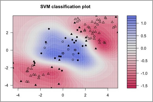
6. Support Vector Machines
Support Vector Machines (SVM) algorithm can be typically used for both classification and regression. For classification tasks, the algorithm creates a hyperplane to separate data into classes. While for regression, the algorithm tries to fit a regression line with minimal error.
Look at the following distribution of data. Here the three classes of data cannot be linearly separated. The boundary curves are non-linear. In such a case, finding the curve’s equation becomes a complex job.
Source: http://uc-r.github.io/svm
The Support Vector Machines (SVM) come in handy in determining the separation boundaries in such situations.
7. Random Forest
Random forest is also a supervised learning algorithm that is flexible for classification and regression. This algorithm is a combination of multiple decision trees which are merged to improve the accuracy of prediction .
The following diagram illustrates how the Random Forest Algorithm works −
8. Gradient Boosting
Gradient boosting combines weak learners(decision trees), to create a strong model. It builds new models that correct errors of the previous ones. The goal of this algorithm is to minimize the loss function. It can be efficiently used for classification and regression tasks.
Advantages of Supervised Learning
Supervised learning algorithms are one of the most popular among the machine learning models. Some benefits are:-
The goal in supervised learning is well-defined, which improves the prediction accuracy.
Models trained using supervised learning are effective at predicting and classification since they use labeled datasets.
It can be highly versatile, i.e., applied to various problems, like spam detection, stock prices, etc.
Disadvantages of Supervised Learning
Though supervised learning is the most used, it comes with certain challenges too. Some of them are:
Supervised learning requires a large amount of labeled data for the model to train effectively. It is practically very difficult to collect such huge data; it is expensive and time-consuming.
Supervised learning cannot predict accurately if the test data is different from the training data.
Accurately labeling the data is complex and requires expertise and effort.
Applications of Supervised learning
Supervised learning models are widely used in many applications in various sectors, including the following-
Image recognition − A model is trained on a labeled dataset of images, where each image is associated with a label. The model is fed with data, which allows it to learn patterns and features. Once trained, the model can now be tested using new, unseen data. This is widely used in applications like facial recognition and object detection.
Predictive analytics − Supervised learning algorithms are used to train labeled historical data, allowing the model to learn patterns and relations between input features and output to identify trends and make accurate predictions. Businesses use this method to make data-driven decisions and enhance strategic planning.
There are various Machine Learning algorithms, techniques and methods that can be used to build models for solving real-life problems by using data. In this chapter, we are going to discuss such different kinds of methods.
There are four main types of machine learning methods classified based on human supervision −
Supervised Learning
Unsupervised Learning
Semi-supervised Learning
Reinforcement Learning
In the next four chapters, we will discuss each of these machine learning models in detail. Here, let’s have a brief overview of these methods:
Supervised Learning
Supervised learning algorithms or methods are the most commonly used ML algorithms. This method or learning algorithm takes the data sample i.e. the training data and its associated output i.e. labels or responses with each data sample during the training process.
The main objective of supervised learning algorithms is to learn an association between input data samples and corresponding outputs after performing multiple training data instances.
For example, we have
x: Input variables and
Y: Output variable
Now, apply an algorithm to learn the mapping function from the input to output as follows −
Y=f(x)
Now, the main objective would be to approximate the mapping function so well that even when we have new input data (x), we can easily predict the output variable (Y) for that new input data.
It is called supervised because the whole process of learning can be thought as it is being supervised by a teacher or supervisor. Examples of supervised machine learning algorithms includes Decision tree, Random Forest, KNN, Logistic Regression etc.
Based on the ML tasks, supervised learning algorithms can be divided into the following two broad classes −
Classification
Regression
Classification
The key objective of classification-based tasks is to predict categorial output labels or responses for the given input data. The output will be based on what the model has learned in the training phase. As we know the categorial output responses means unordered and discrete values, hence each output response will belong to a specific class or category. We will discuss Classification and associated algorithms in detail in the upcoming chapters also.
Classification Models
Followings are some common classification models −
Logistic Regression
Decision Trees
Random Forest
K-nearest Neighbor
Support Vector Machine
Naive Bayes
Linear Discriminant Analysis
Neural Networks
Regression
The key objective of regression-based tasks is to predict output labels or responses, which are continuous numeric values, for the given input data. The output will be based on what the model has learned in its training phase. Basically, regression models use the input data features (independent variables) and their corresponding continuous numeric output values (dependent or outcome variables) to learn specific associations between inputs and corresponding outputs. We will discuss regression and associated algorithms in detail in further chapters.
Regression Models
Followings are some common regression models −
Linear Regression
Ridge regression
Decision Trees
Random Forest
K-nearest Neighbor
Neural Network Regression
Unsupervised Learning
As the name suggests, unsupervised learning is opposite to supervised ML methods or algorithms in which we do not have any supervisor to provide any sort of guidance. Unsupervised learning algorithms are handy in the scenario in which we do not have the liberty, like in supervised learning algorithms, of having pre-labeled training data and we want to extract useful pattern from input data.
For example, it can be understood as follows −
Suppose we have −
x: Input variables, then there would be no corresponding output variable and the algorithms need to discover the interesting pattern in data for learning.
Examples of unsupervised machine learning algorithms includes K-means clustering, K-nearest neighbors etc.
Based on the ML tasks, unsupervised learning algorithms can be divided into the following broad classes −
Clustering
Association
Dimensionality Reduction
Clustering
Clustering methods are one of the most useful unsupervised ML methods. These algorithms used to find similarity as well as relationship patterns among data samples and then cluster those samples into groups having similarity based on features. The real-world example of clustering is to group the customers by their purchasing behavior.
Clustering Models
Followings are some common clustering models −
K-Means Clustering
Hierarchical Clustering
Mean-shift Clustering
DBSCAN Clustering
HDBSCAN Clustering
BIRCH Clustering
Affinity Propagation
Agglomerative Clustering
Association
Another useful unsupervised ML method is Association which is used to analyze large dataset to find patterns which further represents the interesting relationships between various items. It is also termed as Association Rule Mining or Market basket analysis which is mainly used to analyze customer shopping patterns.
Association Models
Followings are some common association models −
Apriori Algorithm
Eclat algorithm
FP-growth algorithm
Dimensionality Reduction
This unsupervised ML method is used to reduce the number of feature variables for each data sample by selecting set of principal or representative features. A question arises here is that why we need to reduce the dimensionality? The reason behind is the problem of feature space complexity which arises when we start analyzing and extracting millions of features from data samples. This problem generally refers to curse of dimensionality. PCA (Principal Component Analysis), K-nearest neighbors and discriminant analysis are some of the popular algorithms for this purpose.
Dimensionality Reduction Models
Followings are some common dimensionality Reduction models −
Principal Component Analysis(PCA)
Autoencoders
Singular value decomposition (SVD)
Anomaly Detection
This unsupervised ML method is used to find out the occurrences of rare events or observations that generally do not occur. By using the learned knowledge, anomaly detection methods would be able to differentiate between anomalous or a normal data point. Some of the unsupervised algorithms like clustering, KNN can detect anomalies based on the data and its features.
Semi-supervised Learning
Semi-supervised learning algorithms or methods are neither fully supervised nor fully unsupervised. They basically fall between the two i.e. supervised and unsupervised learning methods. These kinds of algorithms generally use small supervised learning component i.e. small amount of pre-labeled annotated data and large unsupervised learning component i.e. lots of unlabeled data for training. We can follow any of the following approaches for implementing semi-supervised learning methods −
The first and simple approach is to build the supervised model based on small amount of labeled and annotated data and then build the unsupervised model by applying the same to the large amounts of unlabeled data to get more labeled samples. Now, train the model on them and repeat the process.
The second approach needs some extra efforts. In this approach, we can first use the unsupervised methods to cluster similar data samples, annotate these groups and then use a combination of this information to train the model.
Reinforcement Learning
Reinforcement learning methods are different from previously studied methods and very rarely used also. In this kind of learning algorithms, there would be an agent that we want to train over a period of time so that it can interact with a specific environment. The agent will follow a set of strategies for interacting with the environment and then after observing the environment it will take actions regards the current state of the environment. The following are the main steps of reinforcement learning methods −
Step 1 − First, we need to prepare an agent with some initial set of strategies.
Step 2 − Then observe the environment and its current state.
Step 3 − Next, select the optimal policy regards the current state of the environment and perform important action.
Step 4 − Now, the agent can get corresponding reward or penalty as per accordance with the action taken by it in previous step.
Step 5 − Now, we can update the strategies if it is required so.
Step 6 − At last, repeat steps 2-5 until the agent got to learn and adopt the optimal policies.
Reinforcement Learning Models
Following are some common reinforcement learning algorithms −
Q-learning
Markov Decision Process (MDP)
SARSA
DQN
DDPG
We will discuss each of the above machine learning models in detail in upcoming chapters.
Data preparation is a critical step in the machine learning process, and can have a significant impact on the accuracy and effectiveness of the final model. It requires careful attention to detail and a thorough understanding of the data and the problem at hand.
Let’s discuss how data should be prepared in order to fit right with the model for better accuracy and outcome.
What is Data Preparation?
Data preparation is the process of dealing with raw data i.e, cleaning, organizing and transforming it to align with the machine learning algorithms. Data preparation is a continuous process, and has a huge impact on the performance of machine learning model. Clean and structured data would result in better outcomes.
Importance of Data Preparation
In Machine learning, the model learns from the data that is fed. So, the algorithm can learn efficiently only if the data is organized and perfect. The quality of the data you use for your model can have a significant impact on the performance of the model.
Few aspects that define the importance of data preparation in machine learning are −
Improves model accuracy − Machine learning algorithms reply completely on data. When you provide clean and structured data to models, the outcomes are accurate.
Facilitates Feature Engineering − Data preparation often includes the process of selecting or creating new features to train the model. Hence, data preparation would make feature engineering easy.
Data Quality − Collected data most often would contain inconsistencies, errors and irrelevant information. Hence when tasks like data cleaning, transformation are applied, the data is formatted and neat. This can be used for gaining insights and patterns.
Enables rate of prediction − Prepared data makes it easier to analyze results and would yield accurate outcomes.
Data Preparation Process Steps
Data preparation process involves a sequence of steps that is required to make data suitable for analysis and modeling. The goal of data preparation is to make sure that the data is accurate, complete, and relevant for the analysis.
The following are some of the key steps involved in data preparation −
Data Collection
Data Cleaning
Data Transformation
Data Reduction
Data Splitting
The process shown is not always sequential. You might, for example, split your data before you transform it. You might need to collect more data.
Let’s understand each of the above steps in detail −
Data Collection
Data collection is the first step in the process of machine learning, where data from different sources is gathered to make decisions, answer research questions and statistical planning. Different sources such as databases, text files, pictures, sound files, or web scraping may be used for data collection. Once the data is selected, the data has to be preprocessed in order to gain insights. This process is carried out to put the data in an appropriate format that would be useful for problem solving. Some time data collection follows the data integration step.
Data integration involves combining data from multiple sources into a single dataset for analysis. This may involve matching or linking records across different datasets, or merging datasets based on common variables.
After selecting the raw data, the most important task is data preprocessing. In broad sense, data preprocessing will convert the selected data into a form we can work with or can feed to ML algorithms. We always need to preprocess our data so that it can be as per the expectation of machine learning algorithm. The data preprocessing includes data cleaning, transformation and reduction. Let’s discuss each of these three in detail.
Data Cleaning
Data cleaning is the process of identifying and correcting errors, missing values, duplicate values and outliers, etc. in the data. This step is crucial in the process of machine learning as it ensures that the data is accurate, relevant and error free.
Common techniques used for data cleaning include imputation, outlier detection and removal, etc. The following is a sequence of steps for data cleaning −
1. Handling duplicate values
Duplicates in the dataset means that there is repeated data, which might occur due to data entry errors or issues while collecting data. The technique used to remove duplicates is first they are identified and then deleted using drop_duplicates function in Pandas.
2. Fixing syntax errors
In this step, structural errors like inconsistencies in data format or naming conventions should be addressed. Standardizing formats and fixing errors would ensure data consistence and accurate analysis.
3. Dealing outliers
Outliers are values that are unusual and differ greatly with the data. The techniques used to detect outliers include statistical methods like z-score or IQR method and machine learning methods like clustering and SVM’s.
4. Handling Missing Values
Missing values are the values or data that is not stored for some values in the dataset. There are several ways to handle missing data like:
Imputation − In this process the missing values are substituted with different value, which can be a central tendency measure like mean, median or mode for numeric values and most frequency category for categorical data. Some other methods in imputation include regression imputation and multiple imputation.
Deletion − In this process the entire instances with missing values are removed. Well, this is not a reliable method since there is loss of data.
5. Validating the data
Data Validation is another stage that makes sure that the data aligns perfectly with the requirements so that the predicted outcome is accurate. Some common data validation procedures it the correctness of data before storing them in databases are:
Data type check
Code Check
Format check
Range check
Data Transformation
Data transformation is the process of converting the data from its original format into a format that is suitable for analysis and modeling. This could include defining the structure, aligning the data, extracting data from source, and then storing it in an appropriate form.
There are many techniques available to transorm data into a sutable format. Some commonly used data transformation techniques are as follows −
Scaling
Normalization − L1 & L2 Normalizations
Standardization
Binarization
Encoding
Log Transformation
Lets discuss each of the above data transformation techniques in detail −
1. Scaling
In most cases, the data we collected consists of attributes with varying scale, but we cannot provide such data to ML algorithm hence it requires rescaling. Data scaling makes sure that attributes are at the same scale i.e, usually range of 0 to 1.
We can rescale the data with the help of MinMaxScaler class of scikit-learn Python library.
Example
In this example we will rescale the data of Pima Indians Diabetes dataset which we used earlier. First, the CSV data will be loaded (as done in the previous chapters) and then with the help of MinMaxScaler class, it will be rescaled in the range of 0 and 1.
The first few lines of the following script are same as we have written in previous chapters while loading CSV data.
from pandas import read_csv
from numpy import set_printoptions
from sklearn import preprocessing
path =r'C:\pima-indians-diabetes.csv'
names =['preg','plas','pres','skin','test','mass','pedi','age','class']
dataframe = read_csv(path, names=names)
array = dataframe.values
Now, we can use MinMaxScaler class to rescale the data in the range of 0 and 1.
From the above output, all the data got rescaled into the range of 0 and 1.
2. Normalization
Normalization is used to rescale the data with a distribution value between 0 and 1. For every feature, the minimum value is set to 0 and the maximum value is set to 1.
This is used to rescale each row of data to have a length of 1. It is mainly useful in Sparse dataset where we have lots of zeros. We can rescale the data with the help of Normalizer class of scikit-learn Python library.
In machine learning, there are two types of normalization preprocessing techniques as follows −
L1 Normalization
It may be defined as the normalization technique that modifies the dataset values in a way that in each row the sum of the absolute values will always be up to 1. It is also called Least Absolute Deviations.
Example
In this example, we use L1 Normalize technique to normalize the data of Pima Indians Diabetes dataset which we used earlier. First, the CSV data will be loaded and then with the help of Normalizer class it will be normalized.
The first few lines of following script are same as we have written in previous chapters while loading CSV data.
from pandas import read_csv
from numpy import set_printoptions
from sklearn.preprocessing import Normalizer
path =r'C:\pima-indians-diabetes.csv'
names =['preg','plas','pres','skin','test','mass','pedi','age','class']
dataframe = read_csv (path, names=names)
array = dataframe.values
Now, we can use Normalizer class with L1 to normalize the data.
It may be defined as the normalization technique that modifies the dataset values in a way that in each row the sum of the squares will always be up to 1. It is also called least squares.
Example
In this example, we use L2 Normalization technique to normalize the data of Pima Indians Diabetes dataset which we used earlier. First, the CSV data will be loaded (as done in previous chapters) and then with the help of Normalizer class it will be normalized.
The first few lines of following script are same as we have written in previous chapters while loading CSV data.
from pandas import read_csv
from numpy import set_printoptions
from sklearn.preprocessing import Normalizer
path =r'C:\pima-indians-diabetes.csv'
names =['preg','plas','pres','skin','test','mass','pedi','age','class']
dataframe = read_csv (path, names=names)
array = dataframe.values
Now, we can use Normalizer class with L1 to normalize the data.
Standardization is used to transform data attributes to a standard Gaussian distribution with a mean of 0 and a standard deviation of 1. This technique is useful in ML algorithms like linear regression, logistic regression that assumes a Gaussian distribution in input dataset and produce better results with rescaled data.
We can standardize the data (mean = 0 and SD =1) with the help of StandardScaler class of scikit-learn Python library.
Example
In this example, we will rescale the data of Pima Indians Diabetes dataset which we used earlier. First, the CSV data will be loaded and then with the help of StandardScaler class it will be converted into Gaussian Distribution with mean = 0 and SD = 1.
The first few lines of following script are same as we have written in previous chapters while loading CSV data.
from sklearn.preprocessing import StandardScaler
from pandas import read_csv
from numpy import set_printoptions
path =r'C:\pima-indians-diabetes.csv'
names =['preg','plas','pres','skin','test','mass','pedi','age','class']
dataframe = read_csv(path, names=names)
array = dataframe.values
Now, we can use StandardScaler class to rescale the data.
As the name suggests, this is the technique with the help of which we can make our data binary. We can use a binary threshold for making our data binary. The values above that threshold value will be converted to 1 and below that threshold will be converted to 0. For example, if we choose threshold value = 0.5, then the dataset value above it will become 1 and below this will become 0. That is why we can call it binarizing the data or thresholding the data. This technique is useful when we have probabilities in our dataset and want to convert them into crisp values.
We can binarize the data with the help of Binarizer class of scikit-learn Python library.
Example
In this example, we will rescale the data of Pima Indians Diabetes dataset which we used earlier. First, the CSV data will be loaded and then with the help of Binarizer class it will be converted into binary values i.e. 0 and 1 depending upon the threshold value. We are taking 0.5 as threshold value.
The first few lines of following script are same as we have written in previous chapters while loading CSV data.
from pandas import read_csv
from sklearn.preprocessing import Binarizer
path =r'C:\pima-indians-diabetes.csv'
names =['preg','plas','pres','skin','test','mass','pedi','age','class']
dataframe = read_csv(path, names=names)
array = dataframe.values
Now, we can use Binarize class to convert the data into binary values.
This technique is used to convert categorical variables into numerical representations. Some common encoding techniques include one-hot encoding, label encoding and target encoding.
Label Encoding
Most of the sklearn functions expect that the data with number labels rather than word labels. Hence, we need to convert such labels into number labels. This process is called label encoding. We can perform label encoding of data with the help of LabelEncoder() function of scikit-learn Python library.
Example
In the following example, Python script will perform the label encoding.
First, import the required Python libraries as follows −
import numpy as np
from sklearn import preprocessing
Now, we need to provide the input labels as follows −
This technique is usually used in handling skewed data. It involves apply natural logarithmic function for all values in the dataset to modify the scale of numeric values.
Data Reduction
Data Reduction is a technique to reduce the size of the dataset by selecting a subset of features or observations that are most relevant for the analysis. This can help to reduce noise and improve the accuracy of the model.
This is useful when the dataset is very large or when a dataset contains large amount of irrelevant data.
One of the most common technique used is Dimensionality Reduction, which reduces the size of the dataset without loosing the important information. Other method is the Discretization, where continuous values like time and temperature are converted to discrete categories which simplifies the data.
Data Splitting
Data Splitting is the last step in the preparation of data for machine learning, where the data is split into different sets –
Training − subset which is used by the machine learning model for learning patterns.
Validation − subset used to evaluate the performance of machine learning model while training.
Testing − subset used to evaluate the performance and efficiency of the trained model.
Python Example
Let’s check an example of data preparation using the breast cancer dataset −
from sklearn.datasets import load_breast_cancer
from sklearn.model_selection import train_test_split
from sklearn.preprocessing import StandardScaler

# load the dataset
data = load_breast_cancer()# separate the features and target
X = data.data
y = data.target

# split the data into training and testing sets
X_train, X_test, y_train, y_test = train_test_split(X, y, test_size=0.2, random_state=42)# normalize the data using StandardScaler
scaler = StandardScaler()
X_train = scaler.fit_transform(X_train)
X_test = scaler.transform(X_test)
In this example, we first load the breast cancer dataset using load_breast_cancer function from scikit-learn. Then we separate the features and target, and split the data into training and testing sets using train_test_split function.
Finally, we normalize the data using StandardScaler from scikit-learn, which subtracts the mean and scales the data to unit variance. This helps to bring all the features to a similar scale, which is particularly important for models like SVM and neural networks.
Data Preparation and Feature Engineering
Feature engineering involves creating new features from the existing data that may be more informative or useful for the analysis. It can involve combining or transforming existing features, or creating new features based on domain knowledge or insights. Both data preparation and feature engineering go hand-in-hand in the overall data preprocessing pipeline.
While working with machine learning projects, usually we ignore two most important parts called mathematics and data. What makes data understanding a critical step in ML is its data driven approach. Our ML model will produce only as good or as bad results as the data we provided to it.
Data understanding basically involves analyzing and exploring the data to identify any patterns or trends that may be present.
The data understanding phase typically involves the following steps −
Data Collection − This involves gathering the relevant data that you will be using for your analysis. The data can be collected from various sources such as databases, websites, and APIs.
Data Cleaning − This involves cleaning the data by removing any irrelevant or duplicate data, and dealing with missing data values. The data should be formatted in a way that makes it easy to analyze.
Data Exploration − This involves exploring the data to identify any patterns or trends that may be present. This can be done using various statistical techniques such as histograms, scatter plots, and correlation analysis.
Data Visualization − This involves creating visual representations of the data to help you understand it better. This can be done using tools such as graphs, charts, and maps.
Data Preprocessing − This involves transforming the data to make it suitable for use in machine learning algorithms. This can include scaling the data, transforming it into a different format, or reducing its dimensionality.
Understand the Data before Uploading It in ML Projects
Understanding our data before uploading it into our ML project is important for several reasons −
Identify Data Quality Issues
By understanding your data, you can identify data quality issues such as missing values, outliers, incorrect data types, and inconsistencies that can affect the performance of your ML model. By addressing these issues, you can improve the quality and accuracy of your model.
Determine Data Relevance
You can determine if the data you have collected is relevant to the problem you are trying to solve. By understanding your data, you can determine which features are important for your model and which ones can be ignored.
Select Appropriate ML Techniques
Depending on the characteristics of your data, you may need to choose a particular ML technique or algorithm. For example, if your data is categorical, you may need to use classification techniques, while if your data is continuous, you may need to use regression techniques. Understanding your data can help you select the appropriate ML technique for your problem.
Improve Model Performance
By understanding your data, you can engineer new features, preprocess your data, and select the appropriate ML technique to improve the performance of your model. This can result in better accuracy, precision, recall, and F1 score.
Data Understanding with Statistics
In the previous chapter, we discussed how we can upload CSV data into our ML project, but it would be good to understand the data before uploading it. We can understand the data by two ways, with statistics and with visualization.
In this chapter, with the help of following Python recipes, we are going to understand ML data with statistics.
Looking at Raw Data
The very first recipe is for looking at your raw data. It is important to look at raw data because the insight we will get after looking at raw data will boost our chances to better pre-processing as well as handling of data for ML projects.
Following is a Python script implemented by using head() function of Pandas DataFrame on Pima Indians diabetes dataset to look at the first 10 rows to get better understanding of it −
Example
from pandas import read_csv
path =r"C:\pima-indians-diabetes.csv"
headernames =['preg','plas','pres','skin','test','mass','pedi','age','class']
data = read_csv(path, names=headernames)print(data.head(10))
We can observe from the above output that first column gives the row number which can be very useful for referencing a specific observation.
Checking Dimensions of Data
It is always a good practice to know how much data, in terms of rows and columns, we are having for our ML project. The reasons behind are −
Suppose if we have too many rows and columns then it would take long time to run the algorithm and train the model.
Suppose if we have too less rows and columns then it we would not have enough data to well train the model.
Following is a Python script implemented by printing the shape property on Pandas Data Frame. We are going to implement it on iris data set for getting the total number of rows and columns in it.
Example
from pandas import read_csv
path =r"C:\iris.csv"
data = read_csv(path)print(data.shape)
Output
(150, 4)
We can easily observe from the output that iris data set, we are going to use, is having 150 rows and 4 columns.
Getting Each Attributes Data Type
It is another good practice to know data type of each attribute. The reason behind is that, as per to the requirement, sometimes we may need to convert one data type to another. For example, we may need to convert string into floating point or int for representing categorial or ordinal values. We can have an idea about the attributes data type by looking at the raw data, but another way is to use dtypes property of Pandas DataFrame. With the help of dtypes property we can categorize each attributes data type. It can be understood with the help of following Python script −
Example
from pandas import read_csv
path =r"C:\iris.csv"
data = read_csv(path)print(data.dtypes)
From the above output, we can easily get the datatypes of each attribute.
Statistical Summary of Data
We have discussed Python recipe to get the shape i.e. number of rows and columns, of data but many times we need to review the summaries out of that shape of data. It can be done with the help of describe() function of Pandas DataFrame that further provide the following 8 statistical properties of each & every data attribute −
Count
Mean
Standard Deviation
Minimum Value
Maximum value
25%
Median i.e. 50%
75%
Example
from pandas import read_csv
from pandas import set_option
path =r"C:\pima-indians-diabetes.csv"
names =['preg','plas','pres','skin','test','mass','pedi','age','class']
data = read_csv(path, names=names)
set_option('display.width',100)
set_option('precision',2)print(data.shape)print(data.describe())
From the above output, we can observe the statistical summary of the data of Pima Indian Diabetes dataset along with shape of data.
Reviewing Class Distribution
Class distribution statistics is useful in classification problems where we need to know the balance of class values. It is important to know class value distribution because if we have highly imbalanced class distribution i.e. one class is having lots more observations than other class, then it may need special handling at data preparation stage of our ML project. We can easily get class distribution in Python with the help of Pandas DataFrame.
Example
from pandas import read_csv
path =r"C:\pima-indians-diabetes.csv"
names =['preg','plas','pres','skin','test','mass','pedi','age','class']
data = read_csv(path, names=names)
count_class = data.groupby('class').size()print(count_class)
Output
Class
0  500
1  268
dtype: int64
From the above output, it can be clearly seen that the number of observations with class 0 are almost double than number of observations with class 1.
Reviewing Correlation between Attributes
The relationship between two variables is called correlation. In statistics, the most common method for calculating correlation is Pearsons Correlation Coefficient. It can have three values as follows −
Coefficient value = 1 − It represents full positive correlation between variables.
Coefficient value = -1 − It represents full negative correlation between variables.
Coefficient value = 0 − It represents no correlation at all between variables.
It is always good for us to review the pairwise correlations of the attributes in our dataset before using it into ML project because some machine learning algorithms such as linear regression and logistic regression will perform poorly if we have highly correlated attributes. In Python, we can easily calculate a correlation matrix of dataset attributes with the help of corr() function on Pandas DataFrame.
Example
from pandas import read_csv
from pandas import set_option
path =r"C:\pima-indians-diabetes.csv"
names =['preg','plas','pres','skin','test','mass','pedi','age','class']
data = read_csv(path, names=names)
set_option('display.width',100)
set_option('precision',2)
correlations = data.corr(method='pearson')print(correlations)
The matrix in above output gives the correlation between all the pairs of the attribute in dataset.
Reviewing Skew of Attribute Distribution
Skewness may be defined as the distribution that is assumed to be Gaussian but appears distorted or shifted in one direction or another, or either to the left or right. Reviewing the skewness of attributes is one of the important tasks due to following reasons −
Presence of skewness in data requires the correction at data preparation stage so that we can get more accuracy from our model.
Most of the ML algorithms assumes that data has a Gaussian distribution i.e. either normal of bell curved data.
In Python, we can easily calculate the skew of each attribute by using skew() function on Pandas DataFrame.
Example
from pandas import read_csv
path =r"C:\pima-indians-diabetes.csv"
names =['preg','plas','pres','skin','test','mass','pedi','age','class']
data = read_csv(path, names=names)print(data.skew())
Output
preg   0.90
plas   0.17
pres  -1.84
skin   0.11
test   2.27
mass  -0.43
pedi   1.92
age    1.13
class  0.64
dtype: float64
From the above output, positive or negative skew can be observed. If the value is closer to zero, then it shows less skew.
Suppose if you want to start a ML project then what is the first and most important thing you would require? It is the data that we need to load for starting any of the ML project.
In machine learning, data loading refers to the process of importing or reading data from external sources and converting it into a format that can be used by the machine learning algorithm. The data is then preprocessed to remove any inconsistencies, missing values, or outliers. Once the data is preprocessed, it is split into training and testing sets, which are then used for model training and evaluation.
The data can come from various sources such as CSV files, databases, web APIs, cloud storage, etc. The most common file formats for machine learning projects is CSV (Comma Separated Values).
Consideration While Loading CSV data
CSV is a plain text format that stores tabular data, where each row represents a record, and each column represents a field or attribute. It is widely used because it is simple, lightweight, and can be easily read and processed by programming languages such as Python, R, and Java.
In Python, we can load CSV data into ML projects with different ways but before loading CSV data we must have to take care about some considerations.
In this chapter, let’s understand the main parts of a CSV file, how they might affect the loading and analysis of data, and some consideration we should take care before loading CSV data into ML projects.
File Header
This is the first row of the CSV file, and it typically contains the names of the columns in the table. When loading CSV data into an ML project, the file header (also known as column headers or variable names) can play an important role in data analysis and model training. Here are some considerations to keep in mind regarding the file header −
Consistency − The header row should be consistent across the entire CSV file. This means that the number of columns and their names should be the same for each row. Inconsistencies can cause issues with parsing and analysis.
Meaningful names − Column names should be meaningful and descriptive. This can help with understanding the data and building more accurate models. Avoid using generic names like “column1”, “column2”, etc.
Case sensitivity − Depending on the tool or library being used to load the CSV file, the column names may be case sensitive. It’s important to ensure that the case of the header row matches the expected case sensitivity of the tool or library being used.
Special characters − Column names should not contain any special characters, such as spaces, commas, or quotation marks. These characters can cause issues with parsing and analysis. Instead, use underscores or camelCase to separate words.
Missing header − If the CSV file does not have a header row, it’s important to specify the column names manually or provide a separate file or documentation that includes the column names.
Encoding − The encoding of the header row can affect its interpretation when loading the CSV file. It’s important to ensure that the encoding of the header row is compatible with the tool or library being used to read the file.
Comments
These are optional lines that begin with a specified character, such as “#” or “//”, and are ignored by most programs that read CSV files. They can be used to provide additional information or context about the data in the file.
Comments in a CSV file are not typically used to represent data that would be used in a machine learning project. However, if comments are present in a CSV file, it’s important to consider how they might affect the loading and analysis of the data. Here are some considerations −
Comment markers − In a CSV file, comments can be indicated using a specific marker, such as “#” or “//”. It’s important to know what marker is being used, so that the loading process can ignore comments properly.
Placement − Comments should be placed in a separate line from the actual data. If a comment is included in a line with actual data, it may cause issues with parsing and analysis.
Consistency − If comments are used in a CSV file, it’s important to ensure that the comment marker is used consistently throughout the entire file. Inconsistencies can cause issues with parsing and analysis.
Handling comments − Depending on the tool or library being used to load the CSV file, comments may be ignored by default or may require a specific parameter to be set. It’s important to understand how comments are handled by the tool or library being used.
Effect on analysis − If comments contain important information about the data, it may be necessary to process them separately from the data itself. This can add complexity to the loading and analysis process.
Delimiter
This is the character that separates the fields in each row. While the name suggests that a comma is used as the delimiter, other characters such as tabs, semicolons, or pipes can also be used depending on the file.
The delimiter used in a CSV file can significantly affect the accuracy and performance of a machine learning model, so it is important to consider the following while loading data into an ML project −
Delimiter choice − The delimiter used in a CSV file should be carefully chosen based on the data being used. For example, if the data contains commas within the values (e.g. “New York, NY”), then using a comma as a delimiter may cause issues.In this case, a different delimiter, such as a tab or semicolon, may be more appropriate.
Consistency − The delimiter used in the CSV file should be consistent throughout the entire file. Mixing different delimiters or using whitespace inconsistently can lead to errors and make it difficult to parse the data accurately.
Encoding − The delimiter can also be affected by the encoding of the CSV file. For example, if the CSV file uses a non-ASCII delimiter and is encoded in UTF-8, it may not be correctly read by some machine learning libraries or tools. It is important to ensure that the encoding and delimiter are compatible with the machine learning tools being used.
Other considerations − In some cases, the delimiter may need to be customized based on the machine learning tool being used. For example, some libraries may require a specific delimiter or may not support certain delimiters. It is important to check the documentation of the machine learning tool being used and customize the delimiter as needed.
Quotes
These are optional characters that can be used to enclose fields that contain the delimiter character or newlines. For example, if a field contains a comma, enclosing the field in quotes ensures that the comma is treated as part of the field and not as a delimiter. When loading CSV data into an ML project, there are several considerations to keep in mind regarding the use of quotes −
Quote character − The quote character used in a CSV file should be consistent throughout the file. The most commonly used quote character is the double quote (“) but some files may use single quotes or other characters. It’s important to make sure that the quote character used is consistent with the tool or library being used to read the CSV file.
Quoted values − In some cases, values in a CSV file may be enclosed in quotes to differentiate them from other values. For example, if a field contains a comma, it may be enclosed in quotes to prevent it from being interpreted as a new field. It’s important to make sure that quoted values are properly handled when loading the data into an ML project.
Escaping quotes − If a field contains the quote character used to enclose values, it must be escaped. This is typically done by doubling the quote character. For example, if the quote character is double quote (“) and a field contains the value “John “the Hammer” Smith”, it would be enclosed in quotes and the internal quotes would be escaped like this: “John “”the Hammer”” Smith”.
Use of quotes − The use of quotes in CSV files can vary depending on the tool or library being used to generate the file. Some tools may use quotes around every field, while others may only use quotes around fields that contain special characters. It’s important to make sure that the quote usage is consistent with the tool or library being used to read the file.
Encoding − The use of quotes can also be affected by the encoding of the CSV file. If the file is encoded in a non-standard way, it may cause issues when loading the data into an ML project. It’s important to make sure that the encoding of the CSV file is compatible with the tool or library being used to read the file.
Various Methods of Loading a CSV Data File
While working with ML projects, the most crucial task is to load the data properly into it. As told earlier, the most common data format for ML projects is CSV and it comes in various flavors and varying difficulties to parse.
In this section, we are going to discuss some common approaches in Python to load CSV data file into machine learning project −
Using the CSV Module
This is a built-in module in Python that provides functionality for reading and writing CSV files. You can use it to read a CSV file into a list or dictionary object. Below is its implementation example in Python −
import csv
withopen('mydata.csv','r')asfile:
   reader = csv.reader(file)for row in reader:print(row)
This code reads a CSV file called mydata.csv and prints each row in the file.
Using the Pandas Library
This is a popular data manipulation library in Python that provides a read_csv() function for reading CSV files into a pandas DataFrame object. This is a very convenient way to load data and perform various data manipulation tasks. Below is its implementation example in Python −
import pandas as pd

data = pd.read_csv('mydata.csv')
This code reads a CSV file called mydata.csv and loads it into a pandas DataFrame object called data.
Using the Numpy Library
This is a numerical computing library in Python that provides a genfromtxt() function for loading CSV files into a numpy array. Below is its implementation example in Python −
import numpy as np

data = np.genfromtxt('mydata.csv', delimiter=',')
This code reads a CSV file called mydata.csv and loads it into a numpy array called ‘data’.
Using the Scipy Library
This is a scientific computing library in Python that provides a loadtxt() function for loading text files, including CSV files, into a numpy array. Below is its implementation example in Python −
import numpy as np

from scipy import loadtxt
data = loadtxt('mydata.csv', delimiter=',')
This code reads a CSV file called mydata.csv and loads it into a numpy array called ‘data’.
Using the Sklearn Library
This is a popular machine learning library in Python that provides a load_iris() function for loading the iris dataset, which is a commonly used dataset for classification tasks. Below is its implementation example in Python −
from sklearn.datasets import load_iris

data = load_iris().data
This code loads the iris dataset, which is included in the sklearn library, and loads it into a numpy array called data.
Categorical data in Machine Learning refers to data that consists of categories or labels, rather than numerical values. These categories may be nominal, meaning that there is no inherent order or ranking between them (e.g., color, gender), or ordinal, meaning that there is a natural ordering between the categories (e.g., education level, income bracket).
Categorical data is often represented using discrete values, such as integers or strings, and is frequently encoded as one-hot vectors before being used as input to machine learning models. One-hot encoding involves creating a binary vector for each category, where the vector has a 1 in the position corresponding to the category and 0s in all other positions.
Techniques for Handling Categorical Data
Handling categorical data is an important part of machine learning preprocessing, as many algorithms require numerical input. Depending on the algorithm and the nature of the categorical data, different encoding techniques may be used, such as label encoding, ordinal encoding, or binary encoding etc.
In the subsequent sections of this chapter, we will discuss the following different techniques for handling categorical data in machine learning along with their implementations in Python.
One-Hot Encoding
Label Encoding
Frequency Encoding
Target Encoding
Binary Encoding
Let’s understand the each of the above mentioned techniques to handle categorical data in machine learning.
1. One-Hot Encoding
One-hot encoding is a popular technique for handling categorical data in machine learning. It involves creating a binary vector for each category, where each element of the vector represents the presence or absence of the category. For example, if we have a categorical variable for color with values red, blue, and green, one-hot encoding would create three binary vectors: [1, 0, 0], [0, 1, 0], and [0, 0, 1] respectively.
Example
Below is an example of how to perform one-hot encoding in Python using the Pandas library −
import pandas as pd

# Creating a sample dataset with a categorical variable
data ={'color':['red','green','blue','red','green']}
df = pd.DataFrame(data)# Performing one-hot encoding
one_hot_encoded = pd.get_dummies(df['color'], prefix='color')# Combining the encoded data with the original data
df = pd.concat([df, one_hot_encoded], axis=1)# Drop the original categorical variable
df = df.drop('color', axis=1)# Print the encoded dataprint(df)
Output
This will create a one-hot encoded dataframe with three binary variables (“color_blue,” “color_green,” and “color_red”) that take the value 1 if the corresponding color is present and 0 if it is not. This encoded data, output given below, can then be used for machine learning tasks such as classification and regression.
One-Hot Encoding technique works well for small and finite categorical variables but can be problematic for large categorical variables as it can lead to a high number of input features.
2. Label Encoding
Label Encoding is another technique for handling categorical data in machine learning. It involves assigning a unique numerical value to each category in a categorical variable, with the order of the values based on the order of the categories.
For example, suppose we have a categorical variable “Size” with three categories: “small,” “medium,” and “large.” Using label encoding, we would assign the values 0, 1, and 2 to these categories, respectively.
Example
Below is an example of how to perform label encoding in Python using the scikit-learn library −
from sklearn.preprocessing import LabelEncoder

# create a sample dataset with a categorical variable
data =['small','medium','large','small','large']# create a label encoder object
label_encoder = LabelEncoder()# fit and transform the data using the label encoder
encoded_data = label_encoder.fit_transform(data)# print the encoded dataprint(encoded_data)
This will create an encoded array with the values [0, 1, 2, 0, 2], which correspond to the encoded categories “small,” “medium,” and “large.” Note that the encoding is based on the alphabetical order of the categories by default, but you can change the order by passing a custom list to the LabelEncoder object.
Output
[2 1 0 2 0]
Label encoding can be useful when there is a natural ordering between the categories, such as in the case of ordinal categorical variables. However, it should be used with caution for nominal categorical variables because the numerical values may imply an order that does not actually exist. In these cases, one-hot encoding is a safer option.
3. Frequency Encoding
Frequency Encoding is another technique for handling categorical data in machine learning. It involves replacing each category in a categorical variable with its frequency (or count) in the dataset. The idea behind frequency encoding is that categories that appear more frequently may be more important or informative for the machine learning algorithm.
Example
Below is an example of how to perform frequency encoding in Python −
import pandas as pd

# create a sample dataset with a categorical variable
data ={'color':['red','green','blue','red','green']}
df = pd.DataFrame(data)# calculate the frequency of each category in the categorical variable
freq = df['color'].value_counts(normalize=True)# replace each category with its frequency
df['color_freq']= df['color'].map(freq)# drop the original categorical variable
df = df.drop('color', axis=1)# print the encoded dataprint(df)
This will create an encoded dataframe with one variable (“color_freq”) that represents the frequency of each category in the original categorical variable. For example, if the original variable had two occurrences of “red” and three occurrences of “green,” then the corresponding frequencies would be 0.4 and 0.6, respectively.
Output
      color_freq
0        0.4
1        0.4
2        0.2
3        0.4
4        0.4
Frequency encoding can be a useful alternative to one-hot encoding or label encoding, especially when dealing with high-cardinality categorical variables (i.e., variables with a large number of categories). However, it may not always be effective, and its performance can depend on the particular dataset and machine learning algorithm being used.
4. Target Encoding
Target Encoding is another technique for handling categorical data in machine learning. It involves replacing each category in a categorical variable with the mean (or other aggregation) of the target variable (i.e., the variable you want to predict) for that category. The idea behind target encoding is that it can capture the relationship between the categorical variable and the target variable, and therefore improve the predictive performance of the machine learning model.
Example
Below is an example of how to perform target encoding in Python with the Scikit-learn library by using a combination of a label encoder and a mean encoder −
import pandas as pd
from sklearn.preprocessing import LabelEncoder

# create a sample dataset with a categorical variable and a target variable
data ={'color':['red','green','blue','red','green'],'target':[1,0,1,0,1]}
df = pd.DataFrame(data)# create a label encoder object and fit it to the data
label_encoder = LabelEncoder()
label_encoder.fit(df['color'])# transform the categorical variable using the label encoder
df['color_encoded']= label_encoder.transform(df['color'])# create a mean encoder object and fit it to the transformed data
mean_encoder = df.groupby('color_encoded')['target'].mean().to_dict()# map the mean encoded values to the categorical variable
df['color_encoded']= df['color_encoded'].map(mean_encoder)# print the encoded dataprint(df)
In this example, we first create a Pandas DataFrame df with a categorical variable ‘color’ and a target variable ‘target’. We then create a LabelEncoder object from scikit-learn and fit it to the ‘color’ column of df.
Next, we transform the categorical variable ‘color’ using the label encoder by calling the transform method on the label encoder object and assigning the resulting encoded values to a new column ‘color_encoded‘ in df.
Finally, we create a mean encoder object by grouping df by the ‘color_encoded’ column and calculating the mean of the ‘target’ column for each group. We then convert this mean encoder object to a dictionary and map the mean encoded values to the original ‘color’ column of df.
Output
   color     target     color_encoded
0  red        1           0.5
1  green      0           0.5
2  blue       1           1.0
3  red        0           0.5
4  green      1           0.5
Target encoding can be a powerful technique for improving the predictive performance of machine learning models, especially for datasets with high-cardinality categorical variables. However, it is important to avoid overfitting by using cross-validation and regularization techniques.
5. Binary Encoding
Binary encoding is another technique used for encoding categorical variables in machine learning. In binary encoding, each category is assigned a binary code, where each digit represents whether the category is present (1) or not (0). The binary codes are typically based on the position of the category in a sorted list of all categories.
Example
Here’s an example Python implementation of binary encoding using the category_encoders library −
import pandas as pd
import category_encoders as ce

# create a sample dataset with a categorical variable
data ={'color':['red','green','blue','red','green']}
df = pd.DataFrame(data)# create a binary encoder object and fit it to the data
binary_encoder = ce.BinaryEncoder(cols=['color'])
binary_encoder.fit(df['color'])# transform the categorical variable using the binary encoder
encoded_data = binary_encoder.transform(df['color'])# merge the encoded variable with the original dataframe
df = pd.concat([df, encoded_data], axis=1)# print the encoded dataprint(df)
In this example, we first create a Pandas DataFrame df with a categorical variable ‘color’. We then create a BinaryEncoder object from the category_encoders library and fit it to the ‘color’ column of df.
Next, we transform the categorical variable ‘color’ using the binary encoder by calling the transform method on the binary encoder object and assigning the resulting encoded values to a new DataFrame encoded_data.
Finally, we merge the encoded variable with the original DataFrame df using the concat method along the column axis (axis=1). The resulting DataFrame should have the original ‘color’ column along with the encoded binary columns.
Output
When you run the code, it will produce the following output −
   color    color_0    color_1
0   red       0           1
1   green     1           0
2   blue      1           1
3   red       0           1
4   green     1           0
The binary encoding works best for categorical variables with a moderate number of categories, as it can quickly become inefficient for variables with a large number of categories.