Category: Dimensionality Reduction In ML

Principal Component Analysis (PCA) is a popular unsupervised dimensionality reduction technique in machine learning used to transform high-dimensional data into a lower-dimensional representation. PCA is used to identify patterns and structure in data by discovering the underlying relationships between variables. It is commonly used in applications such as image processing, data compression, and data visualization.

PCA works by identifying the principal components (PCs) of the data, which are linear combinations of the original variables that capture the most variation in the data. The first principal component accounts for the most variance in the data, followed by the second principal component, and so on. By reducing the dimensionality of the data to only the most significant PCs, PCA can simplify the problem and improve the computational efficiency of downstream machine learning algorithms.

The steps involved in PCA are as follows −

• Standardize the data − PCA requires that the data be standardized to have zero mean and unit variance.
• Compute the covariance matrix − PCA computes the covariance matrix of the standardized data.
• Compute the eigenvectors and eigenvalues of the covariance matrix − PCA then computes the eigenvectors and eigenvalues of the covariance matrix.
• Select the principal components − PCA selects the principal components based on their corresponding eigenvalues, which indicate the amount of variation in the data explained by each component.
• Project the data onto the new feature space − PCA projects the data onto the new feature space defined by the selected principal components.

Example

Here is an example of how you can implement PCA in Python using the scikit-learn library −

# Import the necessary librariesimport numpy as np
from sklearn.decomposition import PCA

# Load the iris datasetfrom sklearn.datasets import load_iris
iris = load_iris()# Define the predictor variables (X) and the target variable (y)
X = iris.data
y = iris.target

# Standardize the data
X_standardized =(X - np.mean(X, axis=0))/ np.std(X, axis=0)# Create a PCA object and fit the data
pca = PCA(n_components=2)
X_pca = pca.fit_transform(X_standardized)# Print the explained variance ratio of the selected componentsprint('Explained variance ratio:', pca.explained_variance_ratio_)# Plot the transformed dataimport matplotlib.pyplot as plt
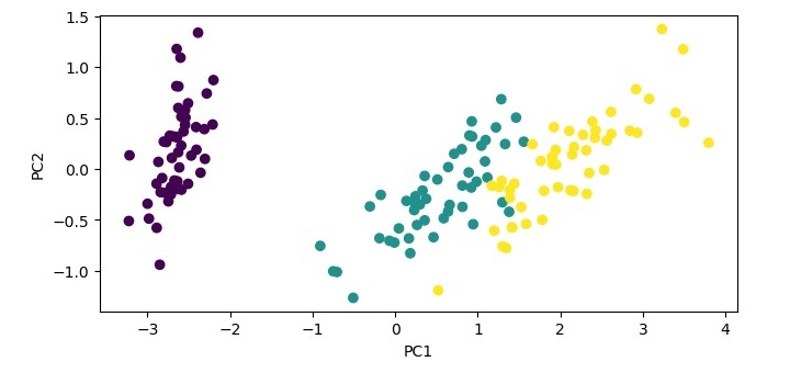
plt.scatter(X_pca[:,0], X_pca[:,1], c=y)
plt.xlabel('PC1')
plt.ylabel('PC2')
plt.show()

In this example, we load the iris dataset, standardize the data, and create a PCA object with two components. We then fit the PCA object to the standardized data and transform the data onto the two principal components. We print the explained variance ratio of the selected components and plot the transformed data using the first two principal components as the x and y axes.

Output

When you execute this code, it will produce the following plot as the output −

Explained variance ratio: [0.72962445 0.22850762]

Advantages of PCA

Following are the advantages of using Principal Component Analysis −

• Reduces dimensionality − PCA is particularly useful for high-dimensional datasets because it can reduce the number of features while retaining most of the original variability in the data.
• Removes correlated features − PCA can identify and remove correlated features, which can help improve the performance of machine learning models.
• Improves interpretability − The reduced number of features can make it easier to interpret and understand the data.
• Reduces overfitting − By reducing the dimensionality of the data, PCA can reduce overfitting and improve the generalizability of machine learning models.
• Speeds up computation − With fewer features, the computation required to train machine learning models is faster.

Disadvantages of PCA

Following are the disadvantages of using Principal Component Analysis −

• Information loss − PCA reduces the dimensionality of the data by projecting it onto a lower-dimensional space, which may lead to some loss of information.
• Can be sensitive to outliers − PCA can be sensitive to outliers, which can have a significant impact on the resulting principal components.
• Interpretability may be reduced − Although PCA can improve interpretability by reducing the number of features, the resulting principal components may be more difficult to interpret than the original features.
• Assumes linearity − PCA assumes that the relationships between the features are linear, which may not always be the case.
• Requires standardization − PCA requires that the data be standardized, which may not always be possible or appropriate.

Missing Values Ratio is a feature selection technique used in machine learning to identify and remove features from the dataset that have a high percentage of missing values. This technique is used to improve the performance of the model by reducing the number of features used for training the model and to avoid the problem of bias caused by missing values.

The Missing Values Ratio works by computing the percentage of missing values for each feature in the dataset and removing the features that have a missing value percentage above a certain threshold. This is done because features with a high percentage of missing values may not be useful for predicting the target variable and can introduce bias into the model.

The steps involved in implementing Missing Values Ratio are as follows −

• Compute the percentage of missing values for each feature in the dataset.
• Set a threshold for the percentage of missing values for the features.
• Remove the features that have a missing value percentage above the threshold.
• Use the remaining features for training the machine learning model.

Example

Here is an example of how you can implement Missing Values Ratio in Python −

# Importing the necessary librariesimport numpy as np

# Load the diabetes dataset
diabetes = np.genfromtxt(r'C:\Users\Leekha\Desktop\diabetes.csv', delimiter=',')# Define the predictor variables (X) and the target variable (y)
X = diabetes[:,:-1]
y = diabetes[:,-1]# Compute the percentage of missing values for each feature
missing_percentages = np.isnan(X).mean(axis=0)# Set the threshold for the percentage of missing values for the features
threshold =0.5# Find the indices of the features with a missing value percentage# above the threshold
high_missing_indices =[i for i, percentage inenumerate(missing_percentages)if percentage > threshold]# Remove the high missing value features from the dataset
X_filtered = np.delete(X, high_missing_indices, axis=1)# Print the shape of the filtered datasetprint('Shape of the filtered dataset:', X_filtered.shape)

The above code performs Missing Values Ratio on the diabetes dataset and removes the features that have a missing value percentage above the threshold.

Output

When you execute this code, it will produce the following output −

Shape of the filtered dataset: (769, 8)

Advantages of Missing Value Ratio

Following are the advantages of using Missing Value Ratio −

• Saves computational resources − With fewer features, the computational resources required to train machine learning models are reduced.
• Improves model performance − By removing features with a high percentage of missing values, the Missing Value Ratio can improve the performance of machine learning models.
• Simplifies the model − With fewer features, the model can be easier to interpret and understand.
• Reduces bias − By removing features with a high percentage of missing values, the Missing Value Ratio can reduce bias in the model.

Disadvantages of Missing Value Ratio

Following are the disadvantages of using Missing Value Ratio −

• Information loss − The Missing Value Ratio can lead to information loss because it removes features that may contain important information.
• Affects non-missing data − Removing features with a high percentage of missing values can sometimes have a negative impact on non-missing data, particularly if the features are important for predicting the dependent variable.
• Impact on the dependent variable − Removing features with a high percentage of missing values can sometimes have a negative impact on the dependent variable, particularly if the features are important for predicting the dependent variable.
• Selection bias − The Missing Value Ratio may introduce selection bias if it removes features that are important for predicting the dependent variable.

Low Variance Filter is a feature selection technique used in machine learning to identify and remove low variance features from the dataset. This technique is used to improve the performance of the model by reducing the number of features used for training the model and to remove the features that have little or no discriminatory power.

The Low Variance Filter works by computing the variance of each feature in the dataset and removing the features that have a variance below a certain threshold. This is done because features with low variance have little or no discriminatory power and are unlikely to be useful for predicting the target variable.

The steps involved in implementing Low Variance Filter are as follows −

• Compute the variance of each feature in the dataset.
• Set a threshold for the variance of the features.
• Remove the features that have a variance below the threshold.
• Use the remaining features for training the machine learning model.

Example

Here is an example to implement Low Variance Filter in Python −

# Importing the necessary librariesimport pandas as pd
import numpy as np

# Load the diabetes dataset
diabetes = pd.read_csv(r'C:\Users\Leekha\Desktop\diabetes.csv')# Define the predictor variables (X) and the target variable (y)
X = diabetes.iloc[:,:-1].values
y = diabetes.iloc[:,-1].values

# Compute the variance of each feature
variances = np.var(X, axis=0)# Set the threshold for the variance of the features
threshold =0.1# Find the indices of the low variance features
low_var_indices = np.where(variances < threshold)# Remove the low variance features from the dataset
X_filtered = np.delete(X, low_var_indices, axis=1)# Print the shape of the filtered datasetprint('Shape of the filtered dataset:', X_filtered.shape)

Output

When you execute this code, it will produce the following output −

Shape of the filtered dataset: (768, 8)

Advantages of Low Variance Filter

Following are the advantages of using Low Variance Filter −

• Reduces overfitting − The Low Variance Filter can help reduce overfitting by removing features that do not contribute much to the prediction of the target variable.
• Saves computational resources − With fewer features, the computational resources required to train machine learning models are reduced.
• Improves model performance − By removing low variance features, the Low Variance Filter can improve the performance of machine learning models.
• Simplifies the model − With fewer features, the model can be easier to interpret and understand.

Disadvantages of Low Variance Filter

Following are the disadvantages of using Low Variance Filter −

• Information loss − The Low Variance Filter can lead to information loss because it removes features that may contain important information.
• Affects non-linear relationships − The Low Variance Filter assumes that the relationships between the features are linear. It may not work well for datasets where the relationships between the features are non-linear.
• Impact on the dependent variable − Removing low variance features can sometimes have a negative impact on the dependent variable, particularly if the features are important for predicting the dependent variable.
• Selection bias − The Low Variance Filter may introduce selection bias if it removes features that are important for predicting the dependent variable.

High Correlation Filter is a feature selection technique used in machine learning to identify and remove highly correlated features from the dataset. This technique is used to improve the performance of the model by reducing the number of features used for training the model and to avoid the problem of multicollinearity, which occurs when two or more predictor variables are highly correlated with each other.

The High Correlation Filter works by computing the correlation between each pair of features in the dataset and removing one of the two features that are highly correlated with each other. This is done by setting a threshold for the correlation coefficient between the features, and removing one of the features if the absolute value of the correlation coefficient is greater than the threshold.

The steps involved in implementing High Correlation Filter are as follows −

• Compute the correlation matrix for the dataset.
• Set a threshold for the correlation coefficient between the features.
• Find the pairs of features that have a correlation coefficient greater than the threshold.
• Remove one of the two features from each pair of highly correlated features.
• Use the remaining features for training the machine learning model.

The advantage of using High Correlation Filter is that it reduces the number of features used for training the model, which in turn reduces the complexity of the model and makes it easier to interpret. Moreover, it helps to avoid the problem of multicollinearity, which can lead to unstable and unreliable estimates of the model parameters.

However, there are some limitations to High Correlation Filter. For example, it may not always select the best set of features for the model, especially if there are non-linear relationships between the features and the target variable. Also, if two features are highly correlated, removing one of them may result in the loss of some important information that was present in the removed feature.

Example

Here is an example to implement High Correlation Filter in Python −

# Importing the necessary librariesimport pandas as pd
import numpy as np

# Load the diabetes dataset
diabetes = pd.read_csv(r'C:\Users\Leekha\Desktop\diabetes.csv')# Define the predictor variables (X) and the target variable (y)
X = diabetes.iloc[:,:-1].values
y = diabetes.iloc[:,-1].values

# Compute the correlation matrix
corr_matrix = np.corrcoef(X, rowvar=False)# Set the threshold for high correlation
threshold =0.8# Find the indices of the highly correlated features
high_corr_indices = np.where(np.abs(corr_matrix)> threshold)# Create a set of feature pairs to be removed
features_to_remove =set()# Iterate over the indices of the highly correlated features and# add them to the set of features to be removedfor i, j inzip(*high_corr_indices):if i != j and(j, i)notin features_to_remove:
      features_to_remove.add((i, j))# Convert the set of feature pairs to a list
features_to_remove =list(features_to_remove)# Remove one of the two features from each pair of highly correlated features
X_filtered = np.delete(X,[j for i, j in features_to_remove], axis=1)# Print the shape of the filtered datasetprint('Shape of the filtered dataset:', X_filtered.shape)

Output

When you execute this code, it will produce the following output −

Shape of the filtered dataset: (768, 8)

Advantages of High Correlation Filter

Following are the advantages of using High Correlation Filter −

• Reduces multicollinearity − The High Correlation Filter can reduce multicollinearity, which occurs when two or more features are highly correlated with each other. Multicollinearity can negatively impact the performance of machine learning models.
• Improves model performance − By removing highly correlated features, the High Correlation Filter can improve the performance of machine learning models.
• Simplifies the model − With fewer features, the model can be easier to interpret and understand.
• Saves computational resources − With fewer features, the computational resources required to train machine learning models are reduced.

Disadvantages of High Correlation Filter

Following are the disadvantages of using High Correlation Filter −

• Information loss − The High Correlation Filter can lead to information loss because it removes features that may contain important information.
• Affects non-linear relationships − The High Correlation Filter assumes that the relationships between the features are linear. It may not work well for datasets where the relationships between the features are non-linear.
• Impact on the dependent variable − Removing highly correlated features can sometimes have a negative impact on the dependent variable, particularly if the features are strongly correlated with the dependent variable.
• Selection bias − The High Correlation Filter may introduce selection bias if it removes features that are important for predicting the dependent variable.

Forward Feature Construction is a feature selection method in machine learning where we start with an empty set of features and iteratively add the best performing feature at each step until the desired number of features is reached.

The goal of feature selection is to identify the most important features that are relevant for predicting the target variable, while ignoring the less important features that add noise to the model and may lead to overfitting.

The steps involved in Forward Feature Construction are as follows −

• Initialize an empty set of features.
• Set the maximum number of features to be selected.
• Iterate until the desired number of features is reached −
  • For each remaining feature that is not already in the set of selected features, fit a model with the selected features and the current feature, and evaluate its performance using a validation set.
  • Select the feature that leads to the best performance and add it to the set of selected features.
• Return the set of selected features as the optimal set for the model.

The key advantage of Forward Feature Construction is that it is computationally efficient and can be used for high-dimensional datasets. However, it may not always lead to the optimal set of features, especially if there are highly correlated features or non-linear relationships between the features and the target variable.

Example

Here is an example to implement Forward Feature Construction in Python −

# Importing the necessary librariesimport pandas as pd
import numpy as np
from sklearn.model_selection import train_test_split
from sklearn.linear_model import LinearRegression
from sklearn.metrics import mean_squared_error

# Load the diabetes dataset
diabetes = pd.read_csv(r'C:\Users\Leekha\Desktop\diabetes.csv')# Define the predictor variables (X) and the target variable (y)
X = diabetes.iloc[:,:-1].values
y = diabetes.iloc[:,-1].values

# Split the data into training and testing sets
X_train, X_test, y_train, y_test = train_test_split(X, y, test_size =0.2, random_state =0)# Create an empty set of features
selected_features =set()# Set the maximum number of features to be selected
max_features =8# Iterate until the desired number of features is reachedwhilelen(selected_features)< max_features:# Set the best feature and the best score to be 0
   best_feature =None
   best_score =0# Iterate over all the remaining featuresfor i inrange(X_train.shape[1]):# Skip the feature if it's already selectedif i in selected_features:continue# Select the current feature and fit a linear regression model
      X_train_selected = X_train[:,list(selected_features)+[i]]
      regressor = LinearRegression()
      regressor.fit(X_train_selected, y_train)# Compute the score on the testing set
      X_test_selected = X_test[:,list(selected_features)+[i]]
      score = regressor.score(X_test_selected, y_test)# Update the best feature and score if the current feature performs betterif score > best_score:
         best_feature = i
         best_score = score

   # Add the best feature to the set of selected features
   selected_features.add(best_feature)# Print the selected features and the scoreprint('Selected Features:',list(selected_features))print('Score:', best_score)

Output

On execution, it will produce the following output −

Selected Features: [1]
Score: 0.23530716168783583
Selected Features: [0, 1]
Score: 0.2923143573608237
Selected Features: [0, 1, 5]
Score: 0.3164103491569179
Selected Features: [0, 1, 5, 6]
Score: 0.3287368302427327
Selected Features: [0, 1, 2, 5, 6]
Score: 0.334586804842275
Selected Features: [0, 1, 2, 3, 5, 6]
Score: 0.3356264736550455
Selected Features: [0, 1, 2, 3, 4, 5, 6]
Score: 0.3313166516703744
Selected Features: [0, 1, 2, 3, 4, 5, 6, 7]
Score: 0.32230203252064216

Backward Elimination is a feature selection technique used in machine learning to select the most significant features for a predictive model. In this technique, we start by considering all the features initially, and then we iteratively remove the least significant features until we get the best subset of features that gives the best performance.

Implementation in Python

To implement Backward Elimination in Python, you can follow these steps −

Import the necessary libraries: pandas, numpy, and statsmodels.api.

import pandas as pd
import numpy as np
import statsmodels.api as sm

Load your dataset into a Pandas DataFrame. We will be using Pima-Indians-Diabetes dataset

diabetes = pd.read_csv(r'C:\Users\Leekha\Desktop\diabetes.csv')

Define the predictor variables (X) and the target variable (y).

X = dataset.iloc[:,:-1].values
y = dataset.iloc[:,-1].values

Add a column of ones to the predictor variables to represent the intercept.

X = np.append(arr = np.ones((len(X),1)).astype(int), values = X, axis =1)

Use the Ordinary Least Squares (OLS) method from the statsmodels library to fit the multiple linear regression model with all the predictor variables.

X_opt = X[:,[0,1,2,3,4,5]]
regressor_OLS = sm.OLS(endog = y, exog = X_opt).fit()

Check the p-values of each predictor variable and remove the one with the highest p-value (i.e., the least significant).

regressor_OLS.summary()

Repeat steps 5 and 6 until all the remaining predictor variables have a p-value below the significance level (e.g., 0.05).

X_opt = X[:,[0,1,3,4,5]]
regressor_OLS = sm.OLS(endog = y, exog = X_opt).fit()
regressor_OLS.summary()

X_opt = X[:,[0,3,4,5]]
regressor_OLS = sm.OLS(endog = y, exog = X_opt).fit()
regressor_OLS.summary()

X_opt = X[:,[0,3,5]]
regressor_OLS = sm.OLS(endog = y, exog = X_opt).fit()
regressor_OLS.summary()

X_opt = X[:,[0,3]]
regressor_OLS = sm.OLS(endog = y, exog = X_opt).fit()
regressor_OLS.summary()

The final subset of predictor variables with p-values below the significance level is the optimal set of features for the model.

Example

Here is the complete implementation of Backward Elimination in Python −

# Importing the necessary librariesimport pandas as pd
import numpy as np
import statsmodels.api as sm

# Load the diabetes dataset
diabetes = pd.read_csv(r'C:\Users\Leekha\Desktop\diabetes.csv')# Define the predictor variables (X) and the target variable (y)
X = diabetes.iloc[:,:-1].values
y = diabetes.iloc[:,-1].values

# Add a column of ones to the predictor variables to represent the intercept
X = np.append(arr = np.ones((len(X),1)).astype(int), values = X, axis =1)# Fit the multiple linear regression model with all the predictor variables
X_opt = X[:,[0,1,2,3,4,5,6,7,8]]
regressor_OLS = sm.OLS(endog = y, exog = X_opt).fit()# Check the p-values of each predictor variable and remove the one# with the highest p-value (i.e., the least significant)
regressor_OLS.summary()# Repeat the above step until all the remaining predictor variables# have a p-value below the significance level (e.g., 0.05)
X_opt = X[:,[0,1,2,3,5,6,7,8]]
regressor_OLS = sm.OLS(endog = y, exog = X_opt).fit()
regressor_OLS.summary()

X_opt = X[:,[0,1,3,5,6,7,8]]
regressor_OLS = sm.OLS(endog = y, exog = X_opt).fit()
regressor_OLS.summary()

X_opt = X[:,[0,1,3,5,7,8]]
regressor_OLS = sm.OLS(endog = y, exog = X_opt).fit()
regressor_OLS.summary()

X_opt = X[:,[0,1,3,5,7]]
regressor_OLS = sm.OLS(endog = y, exog = X_opt).fit()
regressor_OLS.summary()

Output

When you execute this program, it will produce the following output −

Feature extraction is often used in image processing, speech recognition, natural language processing, and other applications where the raw data is high-dimensional and difficult to work with.

Example

Here is an example of how to perform feature extraction using Principal Component Analysis (PCA) on the Iris Dataset using Python −

# Import necessary libraries and datasetfrom sklearn.datasets import load_iris
from sklearn.decomposition import PCA
import matplotlib.pyplot as plt

# Load the dataset
iris = load_iris()# Perform feature extraction using PCA
pca = PCA(n_components=2)
X_pca = pca.fit_transform(iris.data)# Visualize the transformed data
plt.figure(figsize=(7.5,3.5))
plt.scatter(X_pca[:,0], X_pca[:,1], c=iris.target)
plt.xlabel('PC1')
plt.ylabel('PC2')
plt.show()

In this code, we first import the necessary libraries, including sklearn for performing feature extraction using PCA and matplotlib for visualizing the transformed data.

Next, we load the Iris Dataset using load_iris(). We then perform feature extraction using PCA with PCA() and set the number of components to 2 (n_components=2). This reduces the dimensionality of the input data from 4 features to 2 principal components.

We then transform the input data using fit_transform() and store the transformed data in X_pca. Finally, we visualize the transformed data using plt.scatter() and color the data points based on their target value. We label the axes as PC1 and PC2, which are the first and second principal components, respectively, and show the plot using plt.show().

Output

When you execute the given program, it will produce the following plot as the output −

Advantages of Feature Extraction

Following are the advantages of using Feature Extraction −

• Reduced Dimensionality − Feature extraction reduces the dimensionality of the input data by transforming it into a new set of features. This makes the data easier to visualize, process and analyze.
• Improved Performance − Feature extraction can improve the performance of machine learning algorithms by creating a set of more meaningful features that capture the essential information from the input data.
• Feature Selection − Feature extraction can be used to perform feature selection by selecting a subset of the most relevant features that are most informative for the machine learning model.
• Noise Reduction − Feature extraction can also help reduce noise in the data by filtering out irrelevant features or combining related features.

Disadvantages of Feature Extraction

Following are the disadvantages of using Feature Extraction −

• Loss of Information − Feature extraction can result in a loss of information as it involves reducing the dimensionality of the input data. The transformed data may not contain all the information from the original data, and some information may be lost in the process.
• Overfitting − Feature extraction can also lead to overfitting if the transformed features are too complex or if the number of features selected is too high.
• Complexity − Feature extraction can be computationally expensive and time-consuming, especially when dealing with large datasets or complex feature extraction techniques such as deep learning.
• Domain Expertise − Feature extraction requires domain expertise to select and transform the features effectively. It requires knowledge of the data and the problem at hand to choose the right features that are most informative for the machine learning model.

Feature selection is an important step in machine learning that involves selecting a subset of the available features to improve the performance of the model. The following are some commonly used feature selection techniques −

Filter Methods

This method involves evaluating the relevance of each feature by calculating a statistical measure (e.g., correlation, mutual information, chi-square, etc.) and ranking the features based on their scores. Features that have low scores are then removed from the model.

To implement filter methods in Python, you can use the SelectKBest or SelectPercentile functions from the sklearn.feature_selection module. Below is a small code snippet to implement Feature selection.

from sklearn.feature_selection import SelectPercentile, chi2
selector = SelectPercentile(chi2, percentile=10)
X_new = selector.fit_transform(X, y)

Wrapper Methods

This method involves evaluating the model’s performance by adding or removing features and selecting the subset of features that yields the best performance. This approach is computationally expensive, but it is more accurate than filter methods.

To implement wrapper methods in Python, you can use the RFE (Recursive Feature Elimination) function from the sklearn.feature_selection module. Below is a small code snippet to implement Wrapper method.

from sklearn.feature_selection import RFE
from sklearn.linear_model import LogisticRegression

estimator = LogisticRegression()
selector = RFE(estimator, n_features_to_select=5)
selector = selector.fit(X, y)
X_new = selector.transform(X)

Embedded Methods

This method involves incorporating feature selection into the model building process itself. This can be done using techniques such as Lasso regression, Ridge regression, or Decision Trees. These methods assign weights to each feature and features with low weights are removed from the model.

To implement embedded methods in Python, you can use the Lasso or Ridge regression functions from the sklearn.linear_model module. Below is a small code snippet for implementing embedded methods −

from sklearn.linear_model import Lasso

lasso = Lasso(alpha=0.1)
lasso.fit(X, y)
coef = pd.Series(lasso.coef_, index = X.columns)
important_features = coef[coef !=0]

Principal Component Analysis (PCA)

This is a type of unsupervised learning method that involves transforming the original features into a set of uncorrelated principal components that explain the maximum variance in the data. The number of principal components can be selected based on a threshold value, which can reduce the dimensionality of the dataset.

To implement PCA in Python, you can use the PCA function from the sklearn.decomposition module. For example, to reduce the number of features you can use PCA as given the following code −

from sklearn.decomposition import PCA
pca = PCA(n_components=3)
X_new = pca.fit_transform(X)

Recursive Feature Elimination (RFE)

This method involves recursively eliminating the least significant features until a subset of the most important features is identified. It uses a model-based approach and can be computationally expensive, but it can yield good results in high-dimensional datasets.

To implement RFE in Python, you can use the RFECV (Recursive Feature Elimination with Cross Validation) function from the sklearn.feature_selection module. For example, below is a small code snippet with the help of which we can implement to use Recursive Feature Elimination −

from sklearn.feature_selection import RFECV
from sklearn.tree import DecisionTreeClassifier
estimator = DecisionTreeClassifier()
selector = RFECV(estimator, step=1, cv=5)
selector = selector.fit(X, y)
X_new = selector.transform(X)

These feature selection techniques can be used alone or in combination to improve the performance of machine learning models. It is important to choose the appropriate technique based on the size of the dataset, the nature of the features, and the type of model being used.

Example

In the below example, we will implement three feature selection methods − univariate feature selection using the chi-square test, recursive feature elimination with cross-validation (RFECV), and principal component analysis (PCA).

We will use the Breast Cancer Wisconsin (Diagnostic) Dataset, which is included in scikit-learn. This dataset contains 569 samples with 30 features, and the task is to classify whether a tumor is malignant or benign based on these features.

Here is the Python code to implement these feature selection methods on the Breast Cancer Wisconsin (Diagnostic) Dataset −

# Import necessary libraries and datasetimport pandas as pd
from sklearn.datasets import load_diabetes
from sklearn.feature_selection import SelectKBest, chi2
from sklearn.model_selection import train_test_split
from sklearn.linear_model import LogisticRegression

# Load the dataset
diabetes = pd.read_csv(r'C:\Users\Leekha\Desktop\diabetes.csv')# Split the dataset into features and target variable
X = diabetes.drop('Outcome', axis=1)
y = diabetes['Outcome']# Apply univariate feature selection using the chi-square test
selector = SelectKBest(chi2, k=4)
X_new = selector.fit_transform(X, y)# Split the data into training and testing sets
X_train, X_test, y_train, y_test = train_test_split(X_new, y, test_size=0.3, random_state=42)# Fit a logistic regression model on the selected features
clf = LogisticRegression()
clf.fit(X_train, y_train)# Evaluate the model on the test set
accuracy = clf.score(X_test, y_test)print("Accuracy using univariate feature selection: {:.2f}".format(accuracy))# Recursive feature elimination with cross-validation (RFECV)
estimator = LogisticRegression()
selector = RFECV(estimator, step=1, cv=5)
selector.fit(X, y)
X_new = selector.transform(X)
scores = cross_val_score(LogisticRegression(), X_new, y, cv=5)print("Accuracy using RFECV feature selection: %0.2f (+/- %0.2f)"%(scores.mean(), scores.std()*2))# PCA implementation
pca = PCA(n_components=5)
X_new = pca.fit_transform(X)
scores = cross_val_score(LogisticRegression(), X_new, y, cv=5)print("Accuracy using PCA feature selection: %0.2f (+/- %0.2f)"%(scores.mean(), scores.std()*2))

Output

When you execute this code, it will produce the following output on the terminal −

Accuracy using univariate feature selection: 0.74
Accuracy using RFECV feature selection: 0.77 (+/- 0.03)
Accuracy using PCA feature selection: 0.75 (+/- 0.07)

Dimensionality reduction in machine learning is the process of reducing the number of features or variables in a dataset while retaining as much of the original information as possible. In other words, it is a way of simplifying the data by reducing its complexity.

The need for dimensionality reduction arises when a dataset has a large number of features or variables. Having too many features can lead to overfitting and increase the complexity of the model. It can also make it difficult to visualize the data and can slow down the training process.

There are two main approaches to dimensionality reduction −

Feature Selection

This involves selecting a subset of the original features based on certain criteria, such as their importance or relevance to the target variable.

The following are some commonly used feature selection techniques −

• Filter Methods
• Wrapper Methods
• Embedded Methods

Feature Extraction

Feature extraction is a process of transforming raw data into a set of meaningful features that can be used for machine learning models. It involves reducing the dimensionality of the input data by selecting, combining or transforming features to create a new set of features that are more useful for the machine learning model.

Dimensionality reduction can improve the accuracy and speed of machine learning models, reduce overfitting, and simplify data visualization.