Category: Deep Reinforcement Learning

In reinforcement learning, especially in policy optimization techniques, the main goal is to modify the agent’s policy to improve the performance without affecting it’s behavior. This is important when working with deep neural networks, especially if updates are large or not properly limited there might be a case of instability. Trust regions help maintain stability by guaranteeing that parameter updates are smooth and effective during training.

What is Trust Region?

A trust region is a concept used in optimization that restricts updates to the policy or value function in training, maintaining stability and reliability in the learning process. Trust regions assist in limiting the extent to which the model’s parameters, like policy networks, are allowed to vary during updates. This will help in avoiding large or unpredictable changes that may disrupt the learning process.

Role of Trust Regions in Policy Optimization

The idea of trust regions is used to regulate the extent to which the policy can be altered during updates. This guarantees that every update improves the policy without implementing drastic changes that could cause instability or affect performance. Some of the aspects where trust regions play an important role are −

• Policy Gradient − Trust regions are often used in these methods to modify the policy to optimize expected rewards. However, in the absence of a trust region, important updates can result in unpredictable behavior, particularly when employing function approximators such as deep neural networks.
• KL Divergence − This is in Trust Region Policy Optimization (TRPO) which serves as the criteria for evaluating the extent of policy changes by calculating the divergence between the old and new policies. The main concept is that the minor policy changes tend to enhance the agent’s performance consistently, whereas major changes may lead to instability.
• Surrogate Objective in PPO − It is used to estimate the trust region through a surrogate objective function incorporating a clipping mechanism. The primary goal is to prevent major changes in the policy by implementing penalties on big deviations from the previous policy. Additionally, this will improve the performance of the policy.

Trust Region Methods for Deep Reinforcement Learning

Following is a list of algorithms that use trust regions in deep reinforcement learning to ensure that updates are effective and reliable, improving the overall performance −

1. Trust Region Policy Optimization

Trust Region Policy Optimization (TRPO) is a reinforcement learning algorithm that aims to enhance policies in a more efficient and steady way. It deals with the issue of large, unstable updates that usually occur in policy gradient methods by introducing trust region constraint.

The constraint used in TRPO is Kullback-Leibler(KL) divergence, as a restriction to guarantee minimal variation between the old and new policies through the assessment of their disparity. This process helps TRPO in maintaining stability of the learning process and improves the efficiency of the policy.

The TRPO algorithm works by consistently modifying the policy parameters to improve a surrogate objective function with the boundaries of the trust region constraint. For this it is necessary to find a solution for the dilemma of enhancing the policy while maintaining stability.

2. Proximal Policy Optimization

Proximal Policy Optimization is a reinforcement learning algorithm whose aim is to enhance the consistency and dependability of policy updates. This process uses an alternative objective function along with the clipping mechanism to avoid extreme adjustments to policies. This approach ensures that there isn’t much difference between the new policy and old , additionally maintaining a balance between exploration and exploitation.

PPO is an easier and effective among all the trust region techniques. It is widely used in many applications like robotics, autonomous cars because of its reliability and simplicity. The algorithm includes collecting a set of experiences, calculating the advantage estimates, and carrying out several rounds of stochastic gradient descent to modify the policy.

3. Natural Gradient Descent

This technique modifies the step size according to the curvature of the objective function to form a trust region surrounding the current policy. It is particularly effective in high-dimensional environments.

Challenges in Trust Regions

There are certain challenges while implementing trust region techniques in deep reinforcement learning −

• Most trust region techniques like TRPO and PPO require approximations, which can violate constraints or fail to find the optimal solution within the trust region.
• The techniques can be computationally intensive, especially with high-dimensional spaces.
• These techniques often require a wide range of samples for effective learning.
• The efficiency of trust region techniques highly depends on the choice of hyperparameters. Tuning these parameters is quite challenging and often requires expertise.

Deep Deterministic Policy Gradient (DDPG) is an algorithm that simultaneously learns from both Q-function and a policy. It learns the Q-function using off-policy data and the Bellman equation, which is then used to learn the policy.

What is Deep Deterministic Policy Gradient?

Deep Deterministic Policy Gradient (DDPG) is a reinforcement learning algorithm created to address problems with continuous action spaces. This algorithm, which is based on the actor-critic architecture, is off-policy and also a combination of Q-learning and policy gradient methods. DDPG is an off-policy algorithm that is model-free and uses deep learning to estimate value functions and policies, making it suitable for tasks involving continuous actions like robotic control and autonomous driving.

In simple, it expands Deep Q-Networks (DQN) to continuous action spaces with a deterministic policy instead of the usual stochastic policies in DQN or REINFORCE.

Key Concepts in DDPG

The key concepts involved in Deep Deterministic Policy Gradient (DDPG) are −

• Policy Gradient Theorem − The deterministic policy gradient theorem is employed by DDPG, which allows the calculation of the gradient of the expected return in relation to the policy parameters. Additionally, this gradient is used for updating the actor network.
• Off-Policy − DDPG is an off-policy algorithm, indicating it learns from experiences created by a policy that is not the one being optimized. This is done by storing previous experiences in the replay buffer and using them for learning.

What is Deterministic in DDPG?

A deterministic strategy maps states with actions. When you provide a state to the function, it gives back an action to perform. In comparison with the value function, where we obtain probability function for every state. Deterministic policies are used in deterministic environments where the actions taken determine the outcome.

Core Components in DDPG

Following the core components used in Deep Deterministic Policy Gradient (DDPG) −

• Actor-Critic Architecture − While the actor is the policy network, it takes the state as input and outputs a deterministic action. The critic is the Q-function approximator that calculates the action-value function Q(s,a). It considers both the state and the action as input and predicts the expected return.
• Deterministic Policy − DDPG uses deterministic policy instead of stochastic policies, which are mostly used by algorithms like REINFORCE or other policy gradient methods. The actor produces one action for a given state rather than a range of actions.
• Experience Relay − DDPG uses an experience replay buffer for storing previous experiences in tuples consisting of state, action, reward, and next state. The buffer is used for selecting mini-batches in order to break the temporal dependencies among successive experiences, ultimately helping to improve the training stability.
• Target Networks − In order to ensure stability in learning, DDPG employs target networks for both the actor and the critic. These updated versions of the original networks are gradually improved to decrease the variability of updates when training.
• Exploration Noise − Since DDPG is a deterministic policy gradient method, the policy is inherently greedy and would not explore the environment sufficiently.

How does DDPG Work?

Deep Deterministic Policy Gradient (DDPG) is a reinforcement learning algorithm used particularly for continuous action spaces. It is an actor-critic method i.e., it uses two models actor, which decides the action to be taken in the current state and critic, which assesses the effectiveness of the action taken. The working of DDPG is described below −

Continuous Action Spaces

DDPG is effective with environments that have continuous action spaces like controlling the speed and direction of car’s, in contrast to discrete action spaces found in games.

Experience Replay

DDPG uses experience replay by storing the agent’s experiences in a buffer and sampling random batches of experiences for updating the networks. The tuple is represented as (st,at,rt,st+1), where −

• st represents the state at time t.
• at represents the action taken.
• rt represents the reward received.
• st+1 represents the new state after the action.

Randomly selecting experiences from the replay buffer reduces the correlation between consecutive events, leading to more stable training.

Actor-Critic Training

• Critic Update − This critic update is based on Temporal Difference (TD) Learning, particularly the TD(0) variation. The main task of the critic is to assess the actor’s decisions by calculating the Q-value, which predicts the future rewards for specific state-action combinations. Additionally, the critic update in DDPG consists of reducing the TD error (which is the difference between the predicted Q-value and the target Q-value).
• Actor Update − The actor update involves modifying the actor’s neural network to enhance the policy, or decision-making process. In the process of updating the actor, the Q-value gradient is calculated in relation to the action, and the actor’s network is adjusted using gradient ascent to boost the likelihood of choosing actions that result in higher Q-values, enhancing the policy in the end.

Target Networks and Soft Updates

Instead of directly copying learned networks to target networks, DDPG employs a soft update approach, which updates target networks with a portion of the learned networks.

θ′←τ+(1−τ)θ′ where, τ is a small value that ensures slow updates and improves stability.

Exploration-exploitation

DDPG uses Ornstein-Uhlenbeck noise in addition to the actions to promote exploration, as deterministic policies could become trapped in less than ideal solutions with continuous action spaces. The agent is motivated by the noise to explore the environment.

Challenges in DDPG

The two main challenges in DDPG that have to be addressed are −

• Instability − DDPG may experience stability issues in training, especially when employed with function approximators such as neural networks. This is dealt using target networks and experience replay, however, it still needs precise adjustment of hyper parameters.
• Exploration − Even with the use of Ornstein-Uhlenbeck noise for exploration, DDPG could face difficulties in extremely complicated environments if exploration strategies are not effective.

What are Deep Q-Networks?

A Deep Q-Network (DQN) is an algorithm in the field of reinforcement learning. It is a combination of deep neural networks and Q-learning, enabling agents to learn optimal policies in complex environments. While the traditional Q-learning works effectively for environments with a small and finite number of states, but it struggles with large or continuous state spaces due to the size of the Q-table. This limitation is overruled by Deep Q-Networks by replacing the Q-table with neural network that can approximate the Q-values for every state-action pair.

Key Components of Deep Q-Networks

Following is a list of components that are a part of the architecture of Deep Q-Networks −

• Input Layer − This layer receives state information from the environment in the form of a vector of numerical values.
• Hidden Layers − The DQN’s hidden layer consist of multiple fully connected neuron that transform the input data into more complex features that ate more suitable for predictions.
• Output Layer − Each possible action in the current state is represented by a single neuron in the DQN’s output layer. The output values of these neurons represent the estimated value of each action within that state.
• Memory − DQN utilizes a memory replay to store the training events of the agent. All the information including the current state, action taken, the reward received, and the next state are stored as tuples in the memory.
• Loss Function − the DQN computes the difference between the actual Q-values form replay memory and predicted Q-values to determine loss.
• Optimization − It involves adjusting the network’s weights in order to minimize the loss function. Usually, stochastic gradient descent (SGD) is employed for this purpose.

The following image depicts the components in the deep q-network architecture –

How Deep Q-Networks Work?

The working of DQN involves the following steps −

Neural Network Architecture −

The DQN uses a sequence of frames (such as images from a game) for input and generates a set of Q-values for every potential action at that particular state. the typical configuration includes convolutional layers for spatial relationships and fully connected layers for Q-values output.

Experience Replay

While training, the agent stores its interactions (state, action, reward, next state) in a replay buffer. Sampling random batches from this buffer trains the network, reducing correlation between consecutive experiences and improve training stability.

Target Network

In order to stabilize the training process, Deep Q-Networks employ a distinct target network for producing Q-value targets. the target network receives regular updates of weighs from the main network to minimize divergence risk while training.

Epsilon-Greedy Policy

The agent uses an epsilon-greedy strategy, where it selects a random action with probability ϵ and the action with highest Q-value with probability 1−ϵ. This balance between exploration and exploitation helps the agent learn effectively.

Training Process

The neural network is trained using gradient descent to minimize the loss between the predicted Q-values and the target Q-values. The target Q-values are calculated using the Bellman equation, which incorporates the reward received and the maximum Q-value of the nect state.

Limitations of Deep Q-Networks

Deep Q-Networks (DQNs) have several limitations that impacts it’s efficiency and performance −

• DQN’s suffer from instability due to the non-stationarity problem caused from frequent neural network updates.
• DQN’s at times over estimate Q-values, which might have an negative impact on the learning process.
• DQN’s require many samples to learn well, which can be expensive and time-consuming in terms of computation.
• DQN performance is greatly influence by the selection of hyper parameters, such as learning rate, discount factor, and exploration rate.
• DQNs are mainly intended for discrete action spaces and might face difficulties in environments with continuous action spaces.

Double Deep Q-Networks

Double DQN is an extended version of Deep Q-Network created to address an issues in the basic DQN method − Overestimation bias in Q-value updates. The overestimation bias is caused by the fact that the Q-learning update rule utilizes the same Q-network for choosing and assessing actions, resulting in inflated estimates of the Q-values. This problem can cause instability in training and hinder the learning process. The two different networks used in Double DQN to solve this issue −

• Q-Networks, responsible for choosing the action
• Target Network, assess the worth of the chosen action.

The major modification in Double DQN lies in how the target is calculated. Rather than using only Q-network for choosing and assessing the next action, Double DQN involves using the Q-network for selecting the action in the subsequent state and the target network for evaluating the Q-value of the chosen action. This separation decreases the tendency to overestimate and results in more precise value calculations. Due to this, Double DQN offers a more consistent and dependable training process, especially in scenarios such as Atari games, where the regular DQN approach may face challenges with overestimation.

Dueling Deep Q-Networks

Dueling Deep Q-Networks (Dueling DQN), improves the learning process of the traditional Deep Q-Network (DQN) by separating the estimation of state values from action advantages. In the traditional DQN, an individual Q-value is calculated for every state-action combination, representing the expected cumulative reward. However, this can be inefficient, particularly when numerous actions result in similar consequences. Dueling DQN handles this issue by breaking down the Q-value into two primary parts: the state value V(s) and the advantage function A(s,a). The Q-value is then given by Q(s,a)=V(s)+A(s,a), where V(s) captures the value of being in a given state, and A(s,a) measures how much better an action is over others in the same state.

Dueling DQN helps the agent to enhance its understanding of the environment and prevent the learning of unnecessary action-value estimates by separately estimating state values and action advantages. This results in improved performance, particularly in situations with delayed rewards, allowing the agent to gain a better understanding of the importance of various states when choosing the optimal action.

Deep reinforcement learning algorithms are a type of algorithms in machine learning that combines deep learning and reinforcement learning.

Deep reinforcement learning addresses the challenge of enabling computational agents to learn decision-making by incorporating deep learning from unstructured input data without manual engineering of the state space.

Deep reinforcement learning algorithms are capable of deciding what actions to perform for the optimization of an objective even with large inputs.

Reinforcement Learning

Reinforcement Learning consists of an agent that learns from the feedback given in response to its actions while exploring an environment. The main goal of the agent is to maximize cumulative rewards by developing a strategy that guides decision-making in all possible scenarios.

Role of Deep Learning in Reinforcement Learning

In traditional reinforcement learning algorithms, tables or basic function approximates are commonly used to represent value functions, policies, or models. Well, these strategies are not efficient enough to be applied in challenging settings like video games, robotics or natural language processing. Neural networks allow for the approximation of complex, multi-dimensional functions through deep learning. This forms the basis of Deep Reinforcement Learning.

Some of the benefits of the combination of deep learning networks and reinforcement learning are −

• Dealing with inputs with high dimensions (such as raw images and continuous sensor data).
• Understanding complex relationships between states and actions through learning.
• Learning a common representation by generalizing among different states and actions.

Deep Reinforcement Learning Algorithms

The following are some of the common deep reinforcement learning algorithms are −

1. Deep Q-Networks

A Deep Q-Network (DQN) is an extension of conventional Q-learning that employs deep neural networks to estimate the action-value function Q(s,a). Instead of storing Q-values within a table, DQN uses a neural network to deal with complicated input domains like game pixel data. This makes reinforcement learning appropriately address complex tasks, like playing Atari, where the agent learns from visual inputs.

DQN improves training stability through two primary methods: experience replay, which stores and selects past experiences, and target networks to maintain consistent Q-value targets by refreshing a different network periodically. These advancements assist DQN in effectively acquiring knowledge in large-scale settings.

2. Double Deep Q-Networks

Double Deep Q-Network (DDQN) enhances Deep Q-Network (DQN) by mitigating the problem of overestimation bias in Q-value updates. In typical DQN, a single Q-network is utilized for both action selection and value estimation, potentially resulting in overly optimistic value approximations.

DDQN uses two distinct networks to manage action selection and evaluation − a current Q-network for choosing the action and a target Q-network for evaluating the action. This decrease in bias in the Q-value estimates leads to improved learning accuracy. DDQN incorporates the experience replay and target network methods used in DQN to improve the robustness and dependability.

3. Dueling Deep Q-Networks

Dueling Deep Q-Networks (Dueling DQN) is an extension to the standard Deep Q-Network (DQN) used in reinforcement learning. It separates the Q-value into two components − the state value function V(s) and the advantage function A(s,a), which estimates the ratio of the value for each action to the average value.

The final Q-value is estimated by combining all these elements. This form of representation reduces the strength and effectiveness of Q-learning, where the model can estimate the state value more accurately and the need for accurate action values in certain situations is minimized.

4. Policy Gradient Methods

Policy Gradient Methods are algorithms based on a policy iteration approach where policy is directly manipulated to reach the optimal policy that maximizes the expected reward. Rather than focusing on learning a value function, these strategies have been developed in order to maximize rewards by optimizing the policy with respect to the gradient of the defined objective with respect to policy parameters.

The main objective is computing the average reward gradient and strategy modification. The following are the algorithms: REINFORCE, Actor-Critic, and Proximal Policy Optimization (PPO). These approaches can be applied effectively in high or continuous dimensional spaces.

5. Proximal Policy Optimization

A Proximal Policy Optimization (PPO) algorithm in reinforcement learning with an approach to achieve more stable and efficient policy optimization. This approach updates policies by maximizing an objective function associated with the policy, but puts a cap on the amount of allowance for a policy update in order to avoid drastic changes in a policy.

A new policy cannot be too far from an old policy, hence PPO adopts a clipped objective to ensure no policy ever changes drastically from the last policy. By using a clipped objective, PPO will prevent large changes in policy between the old and new one. This balance between the means of exploration and exploitation avoids performance degradation and promotes smoother convergence. PPO is applied in deep reinforcement learning for both continuous and discrete action spaces due to its simplicity and effectiveness.

What is Deep Reinforcement Learning?

Deep Reinforcement Learning (Deep RL) is a subset of Machine Learning that is a combination of reinforcement learning with deep learning. Deep RL addresses the challenge of enabling computational agents to learn decision-making by incorporating deep learning from unstructured input data without manual engineering of the state space. Deep RL algorithms are capable of deciding what actions to perform for the optimization of an objective even with large inputs.

Key Concepts of Deep Reinforcement Learning

The building blocks of Deep Reinforcement Learning include all the aspects that empower learning and agents for decision-making. Effective environments are produced by the collaboration of the following elements −

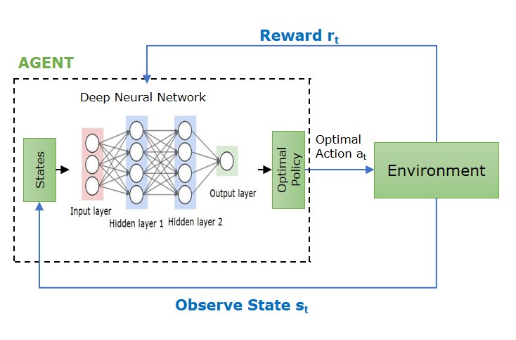
• Agent − The learner and decision-maker who interacts with the environment. This agent acts according to the policies and gains experience.
• Environment − The system outside agent that it communicates with. It gives the agent feedback in the form of incentives or punishments based on its actions.
• State − Represents the current situation or condition of the environment at a specific moment, based on which the agent takes a decision.
• Action − A choice the agent makes that changes the state of the system.
• Policy − A plan that directs the agent’s decision-making by mapping states to actions.
• Value Function − Estimates the expected cumulative reward an agent can achieve from a given state while following a specific policy.
• Model − Represents the environment’s dynamics, allowing the agent to simulate potential outcomes of actions and states for planning purposes.
• Exploration – Exploitation Strategy − A decision-making approach that balances exploring new actions for learning versus exploiting known actions for immediate rewards.
• Learning Algorithm − The method by which the agent updates its value function or policy based on experiences gained from interacting with the environment.
• Experience Replay − A technique that randomly samples from previously stored experiences during training to enhance learning stability and reduce correlations between consecutive events.

How Deep Reinforcement Learning Works?

Deep Reinforcement Learning uses artificial neural networks, which consist of layers of nodes that replicate the functioning of neurons in the human brain. These nodes process and relay information through the trial and error method to determine effective outcomes.

In Deep RL, the term policy refers to the strategy the computer develops based on the feedback it receives from interaction with its environment. These policies help the computer make decisions by considering its current state and the action set, which includes various options. On selecting these options, a process referred to as “search” through which the computer evaluates different actions and observes the outcomes. This ability to coordinate learning, decision-making, and representation could provide new insights simple to how the human brain operates.

Architecture is what sets deep reinforcement learning apart, which allows it to learn similar to the human brain. It contains numerous layers of neural networks that are efficient enough to process unlabeled and unstructured data.

List of Algorithms in Deep RL

Following is the list of some important algorithms in deep reinforcement learning −

• Deep Q-Network or Deep Q-Learning
• Double Deep Q-Learning
• Actor – Critic Method
• Deep Deterministic Policy Gradient

Applications of Deep Reinforcement Learning

Some prominent fields that use deep Reinforcement Learning are −

1. Gaming

Deep RL is used in developing games that are far beyond what is humanly possible. The games designed using Deep RL include Atari 2600 games, Go, Poker, and many more.

2. Robot Control

This used robust adversarial reinforcement learning wherein an agent learns to operate in the presence of an adversary that applies disturbances to the system. The goal is to develop an optimal strategy to handle disruptions. AI-powered robots have a wide range of applications, including manufacturing, supply chain automation, healthcare, and many more.

3. Self-driving Cars

Deep reinforcement learning is one of the key concepts involved in autonomous driving. Autonomous driving scenarios involve understanding the environment, interacting agents, negotiation, and dynamic decision-making, which is possible only by Reinforcement learning.

4. Healthcare

Deep reinforcement learning enabled many advancements in healthcare, like personalization in medication to optimize patient health care, especially for those suffering from chronic conditions.

Difference Between RL and Deep RL

The following table highlights the key differences between Reinforcement Learning(RL) and Deep Reinforcement Learning (Deep RL) −

Feature	Reinforcement Learning	Deep Reinforcement Learning
Definition	It is a subset of Machine Learning that uses trial and error method for decision making.	It is a subset of RL that integrates deep learning for more complex decisions.
Function Approximation	It uses simple methods like tabular methods for value estimation.	It uses neural networks for value estimation, allowing for more complex representation.
State Representation	It relies on manually engineered features to represent the environment.	It automatically learns relevant features from raw input data.
Complexity	It is effective for simple environments with smaller state/action spaces.	It is effective in high-dimensional, complex environments.
Performance	It is effective in simpler environments but struggles in environments with large and continuous spaces.	It excels in complex tasks, including video games or controlling robots.
Applications	Can be used for basic tasks like simple games.	Can be used in advanced applications like autonomous driving, game playing, and robotic control.