Category: Clustering Algorithms In ML

Agglomerative Clustering in Machine Learning

Agglomerative clustering is a hierarchical clustering algorithm that starts with each data point as its own cluster and iteratively merges the closest clusters until a stopping criterion is reached. It is a bottom-up approach that produces a dendrogram, which is a tree-like diagram that shows the hierarchical relationship between the clusters. The algorithm can be implemented using the scikit-learn library in Python.

Agglomerative Clustering Algorithm

Agglomerative Clustering is a hierarchical algorithm that creates a nested hierarchy of clusters by merging clusters in a bottom-up approach. This algorithm includes the following steps −

• Treat each data point as a single cluster
• Compute the proximity matrix using a distance metric
• Merge clusters based on a linkage criterion
• Update the distance matrix
• Repeat steps 3 and 4 until a single cluster remains

Why use Agglomerative Clustering?

The Agglomerative clustering allows easy interpretation of relationships between data points. Unlike k-means clustering, we do not need to specify the number of clusters. It is very efficient and can identify small clusters.

Implementation of Agglomerative Clustering in Python

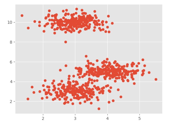
We will use the iris dataset for demonstration. The first step is to import the necessary libraries and load the dataset.

import numpy as np
import pandas as pd
import matplotlib.pyplot as plt
from sklearn.datasets import load_iris
from sklearn.cluster import AgglomerativeClustering
from scipy.cluster.hierarchy import dendrogram, linkage

iris = load_iris()
X = iris.data
y = iris.target

The next step is to create a linkage matrix that contains the distances between each pair of clusters. We can use the linkage function from the scipy.cluster.hierarchy module to create the linkage matrix.

Z = linkage(X,'ward')

The ‘ward’ method is used to calculate the distances between the clusters. It minimizes the variance of the distances between the clusters being merged.

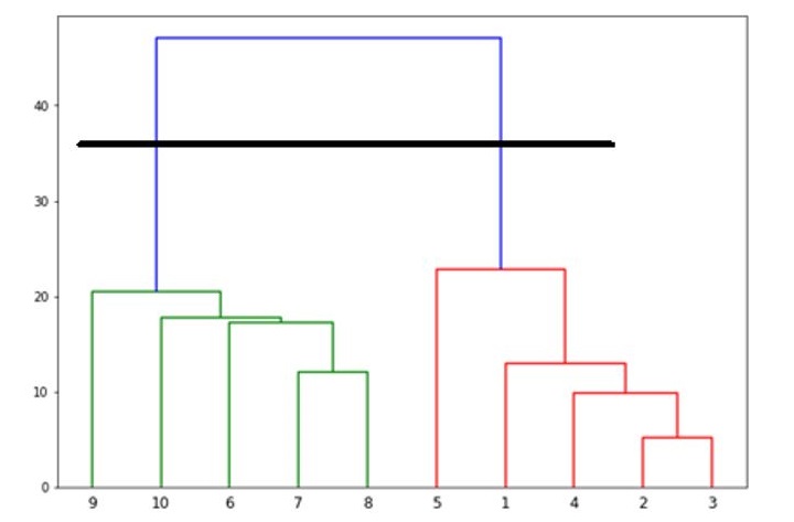
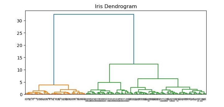
We can visualize the dendrogram using the dendrogram function from the same module.

plt.figure(figsize=(7.5,3.5))
plt.title("Iris Dendrogram")
dendrogram(Z)
plt.show()

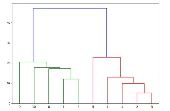
The resulting dendrogram (see the following plot) shows the hierarchical relationship between the clusters. We can see that the algorithm has merged the closest clusters first, and the distance between the clusters increases as we move up the tree.

The final step is to apply the clustering algorithm and extract the cluster labels. We can use the AgglomerativeClustering class from the sklearn.cluster module to apply the algorithm.

model = AgglomerativeClustering(n_clusters=3)
model.fit(X)
labels = model.labels_

The n_clusters parameter specifies the number of clusters to be extracted from the data. In this case, we have specified n_clusters=3 because we know that the iris dataset has three classes.

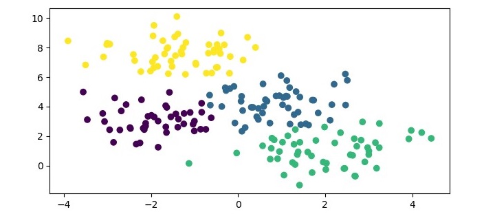
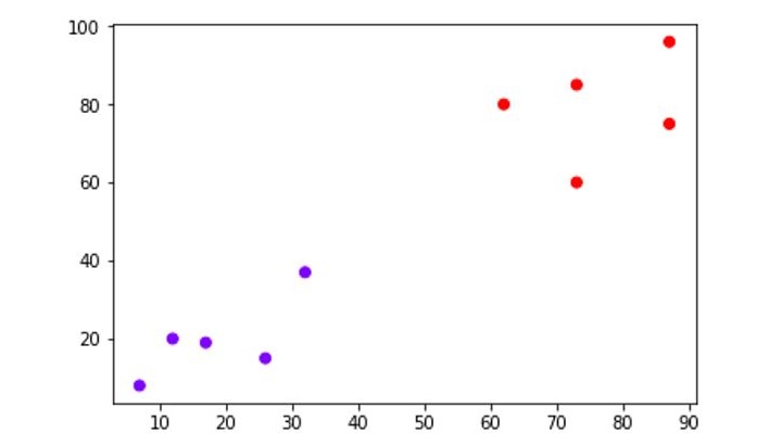
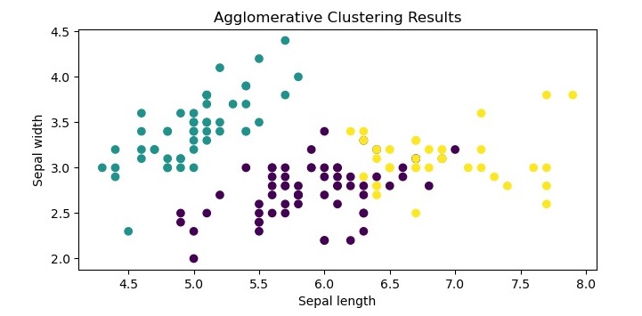
We can visualize the resulting clusters using a scatter plot.

plt.figure(figsize=(7.5,3.5))
plt.scatter(X[:,0], X[:,1], c=labels)
plt.xlabel("Sepal length")
plt.ylabel("Sepal width")
plt.title("Agglomerative Clustering Results")
plt.show()

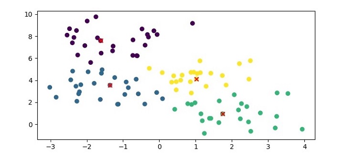
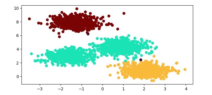
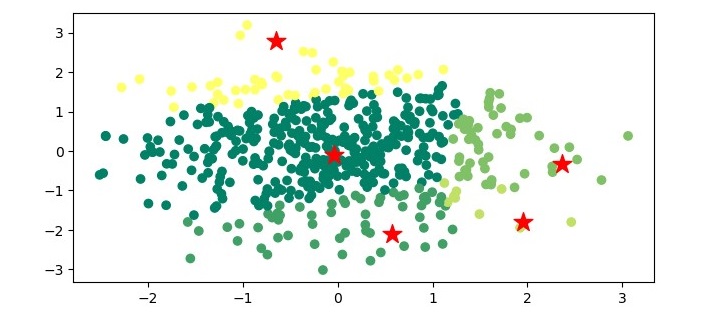
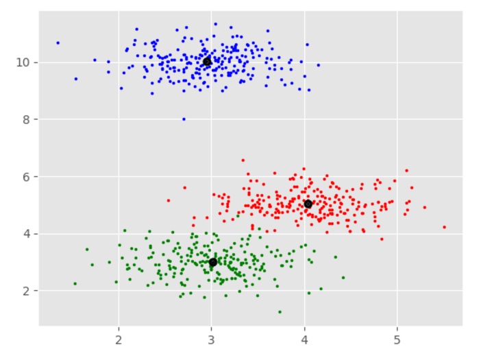
The resulting plot shows the three clusters identified by the algorithm. We can see that the algorithm has successfully separated the data points into their respective classes.

Example

Here is the complete implementation of Agglomerative Clustering in Python −

import numpy as np
import pandas as pd
import matplotlib.pyplot as plt
from sklearn.datasets import load_iris
from sklearn.cluster import AgglomerativeClustering
from scipy.cluster.hierarchy import dendrogram, linkage

# Load the Iris dataset
iris = load_iris()
X = iris.data
y = iris.target
Z = linkage(X,'ward')# Plot the dendogram
plt.figure(figsize=(7.5,3.5))
plt.title("Iris Dendrogram")
dendrogram(Z)
plt.show()# create an instance of the AgglomerativeClustering class
model = AgglomerativeClustering(n_clusters=3)# fit the model to the dataset
model.fit(X)
labels = model.labels_

# Plot the results
plt.figure(figsize=(7.5,3.5))
plt.scatter(X[:,0], X[:,1], c=labels)
plt.xlabel("Sepal length")
plt.ylabel("Sepal width")
plt.title("Agglomerative Clustering Results")
plt.show()

Advantages of Agglomerative Clustering

Following are the advantages of using Agglomerative Clustering −

• Produces a dendrogram that shows the hierarchical relationship between the clusters.
• Can handle different types of distance metrics and linkage methods.
• Allows for a flexible number of clusters to be extracted from the data.
• Can handle large datasets with efficient implementations.

Disadvantages of Agglomerative Clustering

Following are some of the disadvantages of using Agglomerative Clustering −

• Can be computationally expensive for large datasets.
• Can produce imbalanced clusters if the distance metric or linkage method is not appropriate for the data.
• The final result may be sensitive to the choice of distance metric and linkage method used.
• The dendrogram may be difficult to interpret for large datasets with many clusters.

Applications of Agglomerative Clustering

You can find application of Agglomerative Clustering in many areas of unsupervised machine learning tasks. The following are some important areas of its applications in machine learning −

• Image Segmentation
• Document Clustering
• Customer Behaviour Analysis (Customer Segmentation)
• Market Segmentation
• Social Network Analysis

Distribution-based clustering algorithms, also known as probabilistic clustering algorithms, are a class of machine learning algorithms that assume that the data points are generated from a mixture of probability distributions. These algorithms aim to identify the underlying probability distributions that generate the data, and use this information to cluster the data into groups with similar properties.

One common distribution-based clustering algorithm is the Gaussian Mixture Model (GMM). GMM assumes that the data points are generated from a mixture of Gaussian distributions, and aims to estimate the parameters of these distributions, including the means and covariances of each distribution. Let’s see below what is GMM in ML and how we can implement in Python programming language.

Gaussian Mixture Model

Gaussian Mixture Models (GMM) is a popular clustering algorithm used in machine learning that assumes that the data is generated from a mixture of Gaussian distributions. In other words, GMM tries to fit a set of Gaussian distributions to the data, where each Gaussian distribution represents a cluster in the data.

GMM has several advantages over other clustering algorithms, such as the ability to handle overlapping clusters, model the covariance structure of the data, and provide probabilistic cluster assignments for each data point. This makes GMM a popular choice in many applications, such as image segmentation, pattern recognition, and anomaly detection.

Implementation in Python

In Python, the Scikit-learn library provides the GaussianMixture class for implementing the GMM algorithm. The class takes several parameters, including the number of components (i.e., the number of clusters to identify), the covariance type, and the initialization method.

Here is an example of how to implement GMM using the Scikit-learn library in Python −

Example

from sklearn.mixture import GaussianMixture
from sklearn.datasets import make_blobs
import matplotlib.pyplot as plt

# generate a dataset
X, _ = make_blobs(n_samples=200, centers=4, random_state=0)# create an instance of the GaussianMixture class
gmm = GaussianMixture(n_components=4)# fit the model to the dataset
gmm.fit(X)# predict the cluster labels for the data points
labels = gmm.predict(X)# print the cluster labelsprint("Cluster labels:", labels)
plt.figure(figsize=(7.5,3.5))
plt.scatter(X[:,0], X[:,1], c=labels, cmap='viridis')
plt.show()

In this example, we first generate a synthetic dataset using the make_blobs() function from Scikit-learn. We then create an instance of the GaussianMixture class with 4 components and fit the model to the dataset using the fit() method. Finally, we predict the cluster labels for the data points using the predict() method and print the resulting labels.

Output

When you execute this program, it will produce the following plot as the output −

In addition, you will get the following output on the terminal −

Cluster labels: [2 0 1 3 2 1 0 1 1 1 1 2 0 0 2 1 3 3 3 1 3 1 2 0 2 2 3 2 2 1 3 1 0 2 0 1 0
   1 1 3 3 3 3 1 2 0 1 3 3 1 3 0 0 3 2 3 0 2 3 2 3 1 2 1 3 1 2 3 0 0 2 2 1 1
   0 3 0 0 2 2 3 1 2 2 0 1 1 2 0 0 3 3 3 1 1 2 0 3 2 1 3 2 2 3 3 0 1 2 2 1 3
   0 0 2 2 1 2 0 3 1 3 0 1 2 1 0 1 0 2 1 0 2 1 3 3 0 3 3 2 3 2 0 2 2 2 2 1 2
   0 3 3 3 1 0 2 1 3 0 3 2 3 2 2 0 0 3 1 2 2 0 1 1 0 3 3 3 1 3 0 0 1 2 1 2 1
   0 0 3 1 3 2 2 1 3 0 0 0 1 3 1]

The covariance type parameter in GMM controls the type of covariance matrix to use for the Gaussian distributions. The available options include “full” (full covariance matrix), “tied” (tied covariance matrix for all clusters), “diag” (diagonal covariance matrix), and “spherical” (a single variance parameter for all dimensions). The initialization method parameter controls the method used to initialize the parameters of the Gaussian distributions.

Advantages of Gaussian Mixture Models

Following are the advantages of using Gaussian Mixture Models −

• Gaussian Mixture Models (GMM) can model arbitrary distributions of data, making it a flexible clustering algorithm.
• It can handle datasets with missing or incomplete data.
• It provides a probabilistic framework for clustering, which can provide more information about the uncertainty of the clustering results.
• It can be used for density estimation and generation of new data points that follow the same distribution as the original data.
• It can be used for semi-supervised learning, where some data points have known labels and are used to train the model.

Disadvantages of Gaussian Mixture Models

Following are some of the disadvantages of using Gaussian Mixture Models −

• GMM can be sensitive to the choice of initial parameters, such as the number of clusters and the initial values for the means and covariances of the clusters.
• It can be computationally expensive for high-dimensional datasets, as it involves computing the inverse of the covariance matrix, which can be expensive for large matrices.
• It assumes that the data is generated from a mixture of Gaussian distributions, which may not be true for all datasets.
• It may be prone to overfitting, especially when the number of parameters is large or the dataset is small.
• It can be difficult to interpret the resulting clusters, especially when the covariance matrices are complex.

Affinity Propagation is a clustering algorithm that identifies “exemplars” in a dataset and assigns each data point to one of these exemplars. It is a type of clustering algorithm that does not require a pre-specified number of clusters, making it a useful tool for exploratory data analysis. Affinity Propagation was introduced by Frey and Dueck in 2007 and has since been widely used in many fields such as biology, computer vision, and social network analysis.

The idea behind Affinity Propagation is to iteratively update two matrices: the responsibility matrix and the availability matrix. The responsibility matrix contains information about how well-suited each data point is to serve as an exemplar for another data point, while the availability matrix contains information about how much each data point wants to select another data point as an exemplar. The algorithm alternates between updating these two matrices until convergence is achieved. The final exemplars are chosen based on the maximum values in the responsibility matrix.

Implementation in Python

In Python, the Scikit-learn library provides the AffinityPropagation class for implementing the Affinity Propagation algorithm. The class takes several parameters, including the preference parameter, which controls how many exemplars are chosen, and the damping factor, which controls the convergence speed of the algorithm.

Here is an example of how to implement Affinity Propagation using the Scikit-learn library in Python −

Example

from sklearn.cluster import AffinityPropagation
from sklearn.datasets import make_blobs
import matplotlib.pyplot as plt

# generate a dataset
X, _ = make_blobs(n_samples=100, centers=4, random_state=0)# create an instance of the AffinityPropagation class
af = AffinityPropagation(preference=-50)# fit the model to the dataset
af.fit(X)# print the cluster labels and the exemplarsprint("Cluster labels:", af.labels_)print("Exemplars:", af.cluster_centers_indices_)#Plot the result
plt.figure(figsize=(7.5,3.5))
plt.scatter(X[:,0], X[:,1], c=af.labels_, cmap='viridis')
plt.scatter(af.cluster_centers_[:,0], af.cluster_centers_[:,1], marker='x', color='red')
plt.show()

In this example, we first generate a synthetic dataset using the make_blobs() function from Scikit-learn. We then create an instance of the AffinityPropagation class with a preference value of -50 and fit the model to the dataset using the fit() method. Finally, we print the cluster labels and the exemplars identified by the algorithm.

Output

When you execute this code, it will produce the following plot as the output −

In addition, it will print the following output on the terminal −

Cluster labels: [3 0 3 3 3 3 1 0 0 0 0 0 0 0 0 2 3 3 1 2 2 0 1 2 3 1 3 3 2 2 2 0 2 2 1 3 0 2 0 1 3 1 0 1 1 0 2 1 3 1 3 2 1 1 1 0 0 2 2 0 0 2 2 3 2 0 1 1 2 3 0 2 3 0 3 3 3 1 2 2 2 0 1 1 2 1 2 2 3 3 3 1 1 1 1 0 0 1 0 1]
Exemplars: [9 41 51 74]

The preference parameter in Affinity Propagation controls the number of exemplars that are chosen. A higher preference value leads to more exemplars, while a lower preference value leads to fewer exemplars. The damping factor controls the convergence speed of the algorithm, with larger damping factors leading to slower convergence.

Overall, Affinity Propagation is a powerful clustering algorithm that can identify the number of clusters automatically and does not require a pre-specified number of clusters. However, it can be computationally expensive and may not work well with very large datasets.

Advantages of Affinity Propagation

Following are the advantages of using Affinity Propagation −

• Affinity Propagation can identify the number of clusters automatically without specifying the number of clusters in advance.
• It can handle clusters of arbitrary shapes and sizes.
• It can handle datasets with noisy or incomplete data.
• It is relatively insensitive to the choice of initial parameters.
• It has been shown to outperform other clustering algorithms on certain types of datasets.

Disadvantages of Affinity Propagation

Following are some of the disadvantages of using Affinity Propagation −

• It can be computationally expensive for large datasets or datasets with many features.
• It may converge to suboptimal solutions, especially when the data has a high degree of variability or noise.
• It can be sensitive to the choice of the damping factor, which controls the rate of convergence.
• It may produce many small clusters or clusters with only one or a few members, which may not be meaningful.
• It can be difficult to interpret the resulting clusters, as the algorithm does not provide explicit information about the meaning or characteristics of the clusters.

BIRCH (Balanced Iterative Reducing and Clustering hierarchies) is a hierarchical clustering algorithm that is designed to handle large datasets efficiently. The algorithm builds a treelike structure of clusters by recursively partitioning the data into subclusters until a stopping criterion is met.

BIRCH uses two main data structures to represent the clusters: Clustering Feature (CF) and Sub-Cluster Feature (SCF). CF is used to summarize the statistical properties of a set of data points, while SCF is used to represent the structure of subclusters.

BIRCH clustering has three main steps −

• Initialization − BIRCH constructs an empty tree structure and sets the maximum number of CFs that can be stored in a node.
• Clustering − BIRCH reads the data points one by one and adds them to the tree structure. If a CF is already present in a node, BIRCH updates the CF with the new data point. If there is no CF in the node, BIRCH creates a new CF for the data point. BIRCH then checks if the number of CFs in the node exceeds the maximum threshold. If the threshold is exceeded, BIRCH creates a new subcluster by recursively partitioning the CFs in the node.
• Refinement − BIRCH refines the tree structure by merging the subclusters that are similar based on a distance metric.

Implementation of BIRCH Clustering in Python

To implement BIRCH clustering in Python, we can use the scikit-learn library. The scikitlearn library provides a BIRCH class that implements the BIRCH algorithm.

Here is an example of how to use the BIRCH class to cluster a dataset −

Example

from sklearn.datasets import make_blobs
from sklearn.cluster import Birch
import matplotlib.pyplot as plt

# Generate sample data
X, y = make_blobs(n_samples=1000, centers=10, cluster_std=0.50,
random_state=0)# Cluster the data using BIRCH
birch = Birch(threshold=1.5, n_clusters=4)
birch.fit(X)
labels = birch.predict(X)# Plot the results
plt.figure(figsize=(7.5,3.5))
plt.scatter(X[:,0], X[:,1], c=labels, cmap='winter')
plt.show()

In this example, we first generate a sample dataset using the make_blobs function from scikit-learn. We then cluster the dataset using the BIRCH algorithm. For the BIRCH algorithm, we instantiate a Birch object with the threshold parameter set to 1.5 and the n_clusters parameter set to 4. We then fit the Birch object to the dataset using the fit method and predict the cluster labels using the predict method. Finally, we plot the results using a scatter plot.

Output

When you execute the given program, it will produce the following plot as the output −

Advantages of BIRCH Clustering

BIRCH clustering has several advantages over other clustering algorithms, including −

• Scalability − BIRCH is designed to handle large datasets efficiently by using a treelike structure to represent the clusters.
• Memory efficiency − BIRCH uses CF and SCF data structures to summarize the statistical properties of the data points, which reduces the memory required to store the clusters.
• Fast clustering − BIRCH can cluster the data points quickly because it uses an incremental clustering approach.

Disadvantages of BIRCH Clustering

BIRCH clustering also has some disadvantages, including −

• Sensitivity to parameter settings − The performance of BIRCH clustering can be sensitive to the choice of parameters, such as the maximum number of CFs that can be stored in a node and the threshold value used to create subclusters.
• Limited ability to handle non-spherical clusters − BIRCH assumes that the clusters are spherical, which means it may not perform well on datasets with nonspherical clusters.
• Limited flexibility in the choice of distance metric − BIRCH uses the Euclidean distance metric by default, which may not be appropriate for all datasets.

Working of HDBSCAN Clustering

HDBSCAN builds a hierarchy of clusters using a mutual-reachability graph, which is a graph where each data point is a node and the edges between them are weighted by a measure of similarity or distance. The graph is built by connecting two points with an edge if their mutual reachability distance is below a given threshold.

The mutual reachability distance between two points is the maximum of their reachability distances, which is a measure of how easily one point can be reached from the other. The reachability distance between two points is defined as the maximum of their distance and the minimum density of any point along their path.

The hierarchy of clusters is then extracted from the mutual-reachability graph using a minimum spanning tree (MST) algorithm. The leaves of the MST correspond to the individual data points, while the internal nodes correspond to clusters of varying sizes and shapes.

The HDBSCAN algorithm then applies a condensed tree algorithm to the MST to extract the clusters. The condensed tree is a compact representation of the MST that only includes the internal nodes of the tree. The condensed tree is then cut at a certain level to obtain the clusters, with the level of the cut determined by a user-defined minimum cluster size or a heuristic based on the stability of the clusters.

Implementation in Python

HDBSCAN is available as a Python library that can be installed using pip. The library provides an implementation of the HDBSCAN algorithm along with several useful functions for data preprocessing and visualization.

Installation

To install HDBSCAN, open a terminal window and type the following command −

pip install hdbscan

Usage

To use HDBSCAN, first import the hdbscan library −

import hdbscan

Next, we generate a sample dataset using the make_blobs() function from scikit-learn −

# generate random dataset with 1000 samples and 3 clusters
X, y = make_blobs(n_samples=1000, centers=3, random_state=42)

Now, create an instance of the HDBSCAN class and fit it to the data −

clusterer = hdbscan.HDBSCAN(min_cluster_size=10, metric='euclidean')# fit the data to the clusterer
clusterer.fit(X)

This will apply HDBSCAN to the dataset and assign each point to a cluster. To visualize the clustering results, you can plot the data with color each point according to its cluster label −

# get the cluster labels
labels = clusterer.labels_

# create a colormap for the clusters
colors = np.array([x for x in'bgrcmykbgrcmykbgrcmykbgrcmyk'])
colors = np.hstack([colors]*20)# plot the data with each point colored according to its cluster label
plt.figure(figsize=(7.5,3.5))
plt.scatter(X[:,0], X[:,1], c=colors[labels])
plt.show()

This code will produce a scatter plot of the data with each point colored according to its cluster label as follows −

HDBSCAN also provides several parameters that can be adjusted to fine-tune the clustering results −

• min_cluster_size − The minimum size of a cluster. Points that are not part of any cluster are labeled as noise.
• min_samples − The minimum number of samples in a neighborhood for a point to be considered a core point.
• cluster_selection_epsilon − The radius of the neighborhood used for cluster selection.
• metric − The distance metric used to measure the similarity between points.

Advantages of HDBSCAN Clustering

HDBSCAN has several advantages over other clustering algorithms −

• Better handling of clusters of varying densities − HDBSCAN can identify clusters of different densities, which is a common problem in many datasets.
• Ability to detect clusters of different shapes and sizes − HDBSCAN can identify clusters that are not necessarily spherical, which is another common problem in many datasets.
• No need to specify the number of clusters − HDBSCAN does not require the user to specify the number of clusters, which can be difficult to determine a priori.
• Robust to noise − HDBSCAN is robust to noisy data and can identify outliers as noise points.

OPTICS is like DBSCAN (Density-Based Spatial Clustering of Applications with Noise), another popular density-based clustering algorithm. However, OPTICS has several advantages over DBSCAN, including the ability to identify clusters of varying densities, the ability to handle noise, and the ability to produce a hierarchical clustering structure.

Implementation of OPTICS in Python

To implement OPTICS clustering in Python, we can use the scikit-learn library. The scikit-learn library provides a class called OPTICS that implements the OPTICS algorithm.

Here’s an example of how to use the OPTICS class in scikit-learn to cluster a dataset −

Example

from sklearn.cluster import OPTICS
from sklearn.datasets import make_blobs
import matplotlib.pyplot as plt

# Generate sample data
X, y = make_blobs(n_samples=2000, centers=4, cluster_std=0.60, random_state=0)# Cluster the data using OPTICS
optics = OPTICS(min_samples=50, xi=.05)
optics.fit(X)# Plot the results
labels = optics.labels_
plt.figure(figsize=(7.5,3.5))
plt.scatter(X[:,0], X[:,1], c=labels, cmap='turbo')
plt.show()

In this example, we first generate a sample dataset using the make_blobs function from scikit-learn. We then instantiate an OPTICS object with the min_samples parameter set to 50 and the xi parameter set to 0.05. The min_samples parameter specifies the minimum number of samples required for a cluster to be formed, and the xi parameter controls the steepness of the cluster hierarchy. We then fit the OPTICS object to the dataset using the fit method. Finally, we plot the results using a scatter plot, where each data point is colored according to its cluster label.

Output

When you execute this program, it will produce the following plot as the output −

Advantages of OPTICS Clustering

Following are the advantages of using OPTICS clustering −

• Ability to handle clusters of varying densities − OPTICS can handle clusters that have varying densities, unlike some other clustering algorithms that require clusters to have uniform densities.
• Ability to handle noise − OPTICS can identify noise data points that do not belong to any cluster, which is useful for removing outliers from the dataset.
• Hierarchical clustering structure − OPTICS produces a hierarchical clustering structure that can be useful for analyzing the dataset at different levels of granularity.

Disadvantages of OPTICS Clustering

Following are some of the disadvantages of using OPTICS clustering.

• Sensitivity to parameters − OPTICS requires careful tuning of its parameters, such as the min_samples and xi parameters, which can be challenging.
• Computational complexity − OPTICS can be computationally expensive for large datasets, especially when using a high min_samples value.

The DBSCAN Clustering algorithm works as follows −

• Randomly select a data point that has not been visited.
• If the data point has at least minPts neighbors within distance eps, create a new cluster and add the data point and its neighbors to the cluster.
• If the data point does not have at least minPts neighbors within distance eps, mark the data point as noise and continue to the next data point.
• Repeat steps 1-3 until all data points have been visited.

Implementation in Python

We can implement the DBSCAN algorithm in Python using the scikit-learn library. Here are the steps to do so −

Load the dataset

The first step is to load the dataset. We will use the make_moons function from the scikitlearn library to generate a toy dataset with two moons.

from sklearn.datasets import make_moons
X, y = make_moons(n_samples=200, noise=0.05, random_state=0)

Perform DBSCAN clustering

The next step is to perform DBSCAN clustering on the dataset. We will use the DBSCAN class from the scikit-learn library. We will set the minPts parameter to 5 and the “eps” parameter to 0.2.

from sklearn.cluster import DBSCAN
clustering = DBSCAN(eps=0.2, min_samples=5)
clustering.fit(X)

Visualize the results

The final step is to visualize the results of the clustering. We will use the Matplotlib library to create a scatter plot of the dataset colored by the cluster assignments.

import matplotlib.pyplot as plt
plt.scatter(X[:,0], X[:,1], c=clustering.labels_, cmap='rainbow')
plt.show()

Example

Here is the complete implementation of DBSCAN clustering in Python −

from sklearn.datasets import make_moons
X, y = make_moons(n_samples=200, noise=0.05, random_state=0)from sklearn.cluster import DBSCAN

clustering = DBSCAN(eps=0.2, min_samples=5)
clustering.fit(X)import matplotlib.pyplot as plt
plt.figure(figsize=(7.5,3.5))
plt.scatter(X[:,0], X[:,1], c=clustering.labels_, cmap='rainbow')

plt.show()

Output

The resulting scatter plot should show two distinct clusters, each corresponding to one of the moons in the dataset. The noise data points should be colored black.

Advantages of DBSCAN

Following are the advantages of using DBSCAN clustering −

• DBSCAN can handle clusters of arbitrary shape, unlike k-means, which assumes that clusters are spherical.
• It does not require prior knowledge of the number of clusters in the dataset, unlike k-means.
• It can detect outliers, which are points that do not belong to any cluster. This is because DBSCAN defines clusters as dense regions of points, and points that are far from any dense region are considered outliers.
• It is relatively insensitive to the initial choice of parameters, such as the epsilon and min_samples parameters, unlike k-means.
• It is scalable to large datasets, as it only needs to compute pairwise distances between neighboring points, rather than all pairs of points.

Disadvantages of DBSCAN

Following are the disadvantages of using DBSCAN clustering −

• It can be sensitive to the choice of the epsilon and min_samples parameters. If these parameters are not chosen carefully, DBSCAN may fail to identify clusters or merge them incorrectly.
• It may not work well on datasets with varying densities, as it assumes that all clusters have the same density.
• It may produce different results for different runs on the same dataset, due to the non-deterministic nature of the algorithm.
• It may be computationally expensive for high-dimensional datasets, as the distance computations become more expensive as the number of dimensions increases.
• It may not work well on datasets with noise or outliers if the density of the noise or outliers is too high. In such cases, the noise or outliers may be wrongly assigned to clusters.

Density-based clustering is based on the idea that clusters are regions of high density separated by regions of low density.

• The algorithm works by first identifying “core” data points, which are data points that have a minimum number of neighbors within a specified distance. These core data points form the center of a cluster.
• Next, the algorithm identifies “border” data points, which are data points that are not core data points but have at least one core data point as a neighbor.
• Finally, the algorithm identifies “noise” data points, which are data points that are not core data points or border data points.

Popular Density-based Clustering Algorithms

Here are the most common density-based clustering algorithms −

DBSCAN Clustering

The DBSCAN (Density-Based Spatial Clustering of Applications with Noise) algorithm is one of the most common density-based clustering algorithms. The DBSCAN algorithm requires two parameters: the minimum number of neighbors (minPts) and the maximum distance between core data points (eps).

OPTICS Clustering

OPTICS (Ordering Points to Identify the Clustering Structure) is a density-based clustering algorithm that operates by building a reachability graph of the dataset. The reachability graph is a directed graph that connects each data point to its nearest neighbors within a specified distance threshold. The edges in the reachability graph are weighted according to the distance between the connected data points. The algorithm then constructs a hierarchical clustering structure by recursively splitting the reachability graph into clusters based on a specified density threshold.

HDBSCAN Clustering

HDBSCAN (Hierarchical Density-Based Spatial Clustering of Applications with Noise) is a clustering algorithm that is based on density clustering. It is a newer algorithm that builds upon the popular DBSCAN algorithm and offers several advantages over it, such as better handling of clusters of varying densities and the ability to detect clusters of different shapes and sizes.

In the next three chapters, we will discuss all the three density-based clustering algorithms in detail along with their implementation in Python.

Hierarchical Clustering

Hierarchical clustering is an unsupervised learning algorithm that is used to group together the unlabeled data points having similar characteristics. Hierarchical clustering algorithms falls into following two categories −

• Agglomerative hierarchical algorithms − In agglomerative hierarchical algorithms, each data point is treated as a single cluster and then successively merge or agglomerate (bottom-up approach) the pairs of clusters. The hierarchy of the clusters is represented as a dendrogram or tree structure.
• Divisive hierarchical algorithms − On the other hand, in divisive hierarchical algorithms, all the data points are treated as one big cluster and the process of clustering involves dividing (Top-down approach) the one big cluster into various small clusters.

Steps to Perform Agglomerative Hierarchical Clustering

We are going to explain the most used and important Hierarchical clustering i.e. agglomerative. The steps to perform the same is as follows −

• Step 1 − Treat each data point as single cluster. Hence, we will be having say K clusters at start. The number of data points will also be K at start.
• Step 2 − Now, in this step we need to form a big cluster by joining two closet datapoints. This will result in total of K-1 clusters.
• Step 3 − Now, to form more clusters we need to join two closet clusters. This will result in total of K-2 clusters.
• Step 4 − Now, to form one big cluster repeat the above three steps until K would become 0 i.e. no more data points left to join.
• Step 5 − At last, after making one single big cluster, dendrograms will be used to divide into multiple clusters depending upon the problem.

Role of Dendrograms in Agglomerative Hierarchical Clustering

As we discussed in the last step, the role of dendrogram started once the big cluster is formed. Dendrogram will be used to split the clusters into multiple cluster of related data points depending upon our problem. It can be understood with the help of following example −

Example 1

To understand, let’s start with importing the required libraries as follows −

%matplotlib inline
import matplotlib.pyplot as plt
import numpy as np

Next, we will be plotting the datapoints we have taken for this example −

X = np.array([[7,8],[12,20],[17,19],[26,15],[32,37],[87,75],[73,85],[62,80],[73,60],[87,96],])
labels =range(1,11)
plt.figure(figsize=(10,7))
plt.subplots_adjust(bottom=0.1)
plt.scatter(X[:,0],X[:,1], label='True Position')for label, x, y inzip(labels, X[:,0], X[:,1]):
   plt.annotate(label,xy=(x, y), xytext=(-3,3),textcoords='offset points', ha='right', va='bottom')
plt.show()

Output

When you execute this code, it will produce the following plot as the output −

From the above diagram, it is very easy to see we have two clusters in our datapoints but in real-world data, there can be thousands of clusters.

Next, we will be plotting the dendrograms of our datapoints by using Scipy library −

from scipy.cluster.hierarchy import dendrogram, linkage
from matplotlib import pyplot as plt
linked = linkage(X,'single')
labelList =range(1,11)
plt.figure(figsize=(10,7))

dendrogram(linked, orientation='top',labels=labelList,
distance_sort='descending',show_leaf_counts=True)

plt.show()

It will produce the following plot −

Now, once the big cluster is formed, the longest vertical distance is selected. A vertical line is then drawn through it as shown in the following diagram. As the horizontal line crosses the blue line at two points hence the number of clusters would be two.

Next, we need to import the class for clustering and call its fit_predict method to predict the cluster. We are importing AgglomerativeClustering class of sklearn.cluster library −

from sklearn.cluster import AgglomerativeClustering

cluster = AgglomerativeClustering(n_clusters=2, affinity='euclidean',
linkage='ward')

cluster.fit_predict(X)

Next, plot the cluster with the help of following code −

plt.scatter(X[:,0],X[:,1], c=cluster.labels_, cmap='rainbow')

The following diagram shows the two clusters from our datapoints.

Example 2

As we understood the concept of dendrograms from the simple example above, let’s move to another example in which we are creating clusters of the data point in Pima Indian Diabetes Dataset by using hierarchical clustering −

import matplotlib.pyplot as plt
import pandas as pd
%matplotlib inline
import numpy as np

from pandas import read_csv
path =r"C:\pima-indians-diabetes.csv"
headernames =['preg','plas','pres','skin','test','mass','pedi','age','class']
data = read_csv(path, names=headernames)
array = data.values
X = array[:,0:8]
Y = array[:,8]

patient_data = data.iloc[:,3:5].values
import scipy.cluster.hierarchy as shc
plt.figure(figsize=(10,7)) 
plt.title("Patient Dendograms")

dend = shc.dendrogram(shc.linkage(data, method='ward'))from sklearn.cluster import AgglomerativeClustering
cluster = AgglomerativeClustering(n_clusters=4, affinity='euclidean', linkage='ward')
cluster.fit_predict(patient_data)

plt.figure(figsize=(7.2,5.5))
plt.scatter(patient_data[:,0], patient_data[:,1], c=cluster.labels_,
cmap='rainbow')

Output

When you run this code, it will produce the following two plots as the output −

Mean-Shift Clustering Algorithm

The Mean-Shift clustering algorithm is a non-parametric clustering algorithm that works by iteratively shifting the mean of a data point towards the densest area of the data. The densest area of the data is determined by the kernel function, which is a function that assigns weights to the data points based on their distance from the mean. The kernel function used in Mean-Shift clustering is usually a Gaussian function.

The Mean-Shift clustering algorithm is a powerful clustering algorithm used in unsupervised learning. Unlike K-means clustering, it does not make any assumptions; hence it is a non-parametric algorithm.

The difference between K-Means algorithm and Mean-Shift is that later one does not need to specify the number of clusters in advance because the number of clusters will be determined by the algorithm w.r.t data.

Working of Mean-Shift Algorithm

We can understand the working of Mean-Shift clustering algorithm with the help of following steps −

• Step 1 − First, start with the data points assigned to a cluster of their own.
• Step 2 − Next, this algorithm will compute the centroids.
• Step 3 − In this step, location of new centroids will be updated.
• Step 4 − Now, the process will be iterated and moved to the higher density region.
• Step 5 − At last, it will be stopped once the centroids reach at position from where it cannot move further.

The Mean-Shift clustering algorithm is a density-based clustering algorithm, which means that it identifies clusters based on the density of the data points rather than the distance between them. In other words, the algorithm identifies clusters based on the areas where the density of the data points is highest.

Implementation of Mean-Shift Clustering in Python

The Mean-Shift clustering algorithm can be implemented in Python programming language using the scikit-learn library. The scikit-learn library is a popular machine learning library in Python that provides various tools for data analysis and machine learning. The following steps are involved in implementing the Mean-Shift clustering algorithm in Python using the scikit-learn library −

Step 1 − Import the necessary libraries

The numpy library is used for scientific computing in Python, while the matplotlib library is used for data visualization. The sklearn.cluster library contains the MeanShift class, which is used for implementing the Mean-Shift clustering algorithm in Python.

The estimate_bandwidth function is used to estimate the bandwidth of the kernel function, which is an important parameter in the Mean-Shift clustering algorithm.

import numpy as np
import matplotlib.pyplot as plt
from sklearn.cluster import MeanShift, estimate_bandwidth

Step 2 − Generate the data

In this step, we generate a random dataset with 500 data points and 2 features. We use the numpy.random.randn function to generate the data.

# Generate the data
X = np.random.randn(500,2)

Step 3 − Estimate the bandwidth of the kernel function

In this step, we estimate the bandwidth of the kernel function using the estimate_bandwidth function. The bandwidth is an important parameter in the Mean-Shift clustering algorithm, which determines the width of the kernel function.

# Estimate the bandwidth
bandwidth = estimate_bandwidth(X, quantile=0.1, n_samples=100)

Step 4 − Initialize the Mean-Shift clustering algorithm

In this step, we initialize the Mean-Shift clustering algorithm using the MeanShift class. We pass the bandwidth parameter to the class to set the width of the kernel function.

# Initialize the Mean-Shift algorithm
ms = MeanShift(bandwidth=bandwidth, bin_seeding=True)

Step 5 − Train the model

In this step, we train the Mean-Shift clustering algorithm on the dataset using the fit method of the MeanShift class.

# Train the model
ms.fit(X)

Step 6 − Visualize the results

# Visualize the results
labels = ms.labels_
cluster_centers = ms.cluster_centers_
n_clusters_ =len(np.unique(labels))print("Number of estimated clusters:", n_clusters_)# Plot the data points and the centroids
plt.figure(figsize=(7.5,3.5))
plt.scatter(X[:,0], X[:,1], c=labels, cmap='viridis')
plt.scatter(cluster_centers[:,0], cluster_centers[:,1], marker='*', s=300, c='r')
plt.show()

In this step, we visualize the results of the Mean-Shift clustering algorithm. We extract the cluster labels and the cluster centers from the trained model. We then print the number of estimated clusters. Finally, we plot the data points and the centroids using the matplotlib library.

Complete Example

Here is the complete implementation example of Mean-Shift Clustering Algorithm in python −

import numpy as np
import matplotlib.pyplot as plt
from sklearn.cluster import MeanShift, estimate_bandwidth

# Generate the data
X = np.random.randn(500,2)# Estimate the bandwidth
bandwidth = estimate_bandwidth(X, quantile=0.1, n_samples=100)# Initialize the Mean-Shift algorithm
ms = MeanShift(bandwidth=bandwidth, bin_seeding=True)# Train the model
ms.fit(X)# Visualize the results
labels = ms.labels_
cluster_centers = ms.cluster_centers_
n_clusters_ =len(np.unique(labels))print("Number of estimated clusters:", n_clusters_)# Plot the data points and the centroids
plt.figure(figsize=(7.5,3.5))
plt.scatter(X[:,0], X[:,1], c=labels, cmap='summer')
plt.scatter(cluster_centers[:,0], cluster_centers[:,1], marker='*',
s=200, c='r')
plt.show()

Output

When you execute the program, it will produce the following plot as the output −

Example

It is a simple example to understand how Mean-Shift algorithm works. In this example, we are going to first generate 2D dataset containing 4 different blobs and after that will apply Mean-Shift algorithm to see the result.

%matplotlib inline
import numpy as np
from sklearn.cluster import MeanShift
import matplotlib.pyplot as plt
from matplotlib import style
style.use("ggplot")from sklearn.datasets import make_blobs
centers =[[3,3,3],[4,5,5],[3,10,10]]
X, _ = make_blobs(n_samples =700, centers = centers, cluster_std =0.5)
plt.scatter(X[:,0],X[:,1])
plt.show()

Output

ms = MeanShift()
ms.fit(X)
labels = ms.labels_
cluster_centers = ms.cluster_centers_
print(cluster_centers)
n_clusters_ =len(np.unique(labels))print("Estimated clusters:", n_clusters_)
colors =10*['r.','g.','b.','c.','k.','y.','m.']for i inrange(len(X)):
    plt.plot(X[i][0], X[i][1], colors[labels[i]], markersize =3)
plt.scatter(cluster_centers[:,0],cluster_centers[:,1],
    marker=".",color='k', s=20, linewidths =5, zorder=10)
plt.show()

Output

[[ 4.03457771  5.03063843  4.92928409]
 [ 3.01124859  2.9957586   2.981767  ]
 [ 2.94969928 10.00712673 10.01575558]]
Estimated clusters: 3

Applications of Mean-Shift Clustering

The Mean-Shift clustering algorithm has several applications in various fields. Some of the applications of Mean-Shift clustering are as follows −

• Computer vision − Mean-Shift clustering is widely used in computer vision for object tracking, image segmentation, and feature extraction.
• Image processing − Mean-Shift clustering is used for image segmentation, which is the process of dividing an image into multiple segments based on the similarity of the pixels.
• Anomaly detection − Mean-Shift clustering can be used for detecting anomalies in data by identifying the areas with low density.
• Customer segmentation − Mean-Shift clustering can be used for customer segmentation in marketing by identifying groups of customers with similar behavior and preferences.
• Social network analysis − Mean-Shift clustering can be used for clustering users in social networks based on their interests and interactions.

Advantages and Disadvantages

Let’s discuss some advantages and disadvantages of the means-shift clustering algorithm.

Advantages

The following are some advantages of Mean-Shift clustering algorithm −

• It does not need to make any model assumption as like in K-means or Gaussian mixture.
• It can also model the complex clusters which have nonconvex shape.
• It only needs one parameter named bandwidth which automatically determines the number of clusters.
• There is no issue of local minima as like in K-means.
• No problem generated from outliers.

Disadvantages

The following are some disadvantages of Mean-Shift clustering algorithm −

• Mean-shift algorithm does not work well in case of high dimension, where number of clusters changes abruptly.
• We do not have any direct control on the number of clusters but in some applications, we need a specific number of clusters.
• It cannot differentiate between meaningful and meaningless modes.