Merge a set of sorted files of different length into a single sorted file. We need to find an optimal solution, where the resultant file will be generated in minimum time.
If the number of sorted files are given, there are many ways to merge them into a single sorted file. This merge can be performed pair wise. Hence, this type of merging is called as 2-way merge patterns.
As, different pairings require different amounts of time, in this strategy we want to determine an optimal way of merging many files together. At each step, two shortest sequences are merged.
To merge a p-record file and a q-record file requires possibly p + q record moves, the obvious choice being, merge the two smallest files together at each step.
Two-way merge patterns can be represented by binary merge trees. Let us consider a set of n sorted files {f1, f2, f3, , fn}. Initially, each element of this is considered as a single node binary tree. To find this optimal solution, the following algorithm is used.
Pseudocode
Following is the pseudocode of the Optimal Merge Pattern Algorithm −
 for i := 1 to n  1 do
   declare new node
   node.leftchild := least (list)
   node.rightchild := least (list)
   node.weight) := ((node.leftchild).weight)+
   ((node.rightchild).weight)
   insert (list, node);
return least (list);
At the end of this algorithm, the weight of the root node represents the optimal cost.
Examples
Let us consider the given files, f1, f2, f3, f4 and f5 with 20, 30, 10, 5 and 30 number of elements respectively.
If merge operations are performed according to the provided sequence, then
M1 = merge f1 and f2 => 20 + 30 = 50
M2 = merge M1 and f3 => 50 + 10 = 60
M3 = merge M2 and f4 => 60 + 5 = 65
M4 = merge M3 and f5 => 65 + 30 = 95
Hence, the total number of operations is
50 + 60 + 65 + 95 = 270
Now, the question arises is there any better solution?
Sorting the numbers according to their size in an ascending order, we get the following sequence −
f4, f3, f1, f2, f5
Hence, merge operations can be performed on this sequence
M1 = merge f4 and f3 => 5 + 10 = 15
M2 = merge M1 and f1 => 15 + 20 = 35
M3 = merge M2 and f2 => 35 + 30 = 65
M4 = merge M3 and f5 => 65 + 30 = 95
Therefore, the total number of operations is
15 + 35 + 65 + 95 = 210
Obviously, this is better than the previous one.
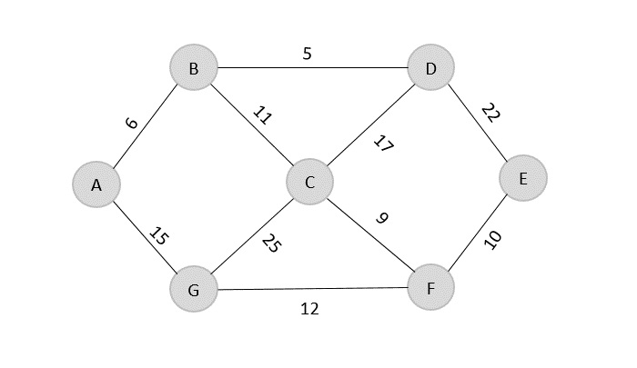
In this context, we are now going to solve the problem using this algorithm.
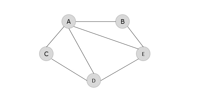
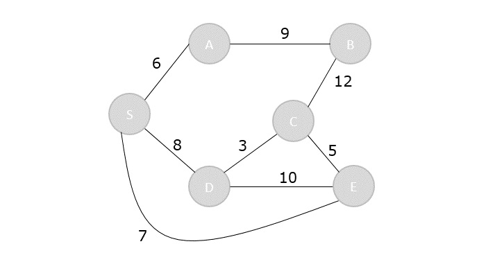
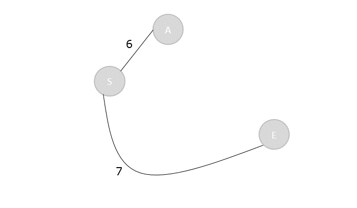
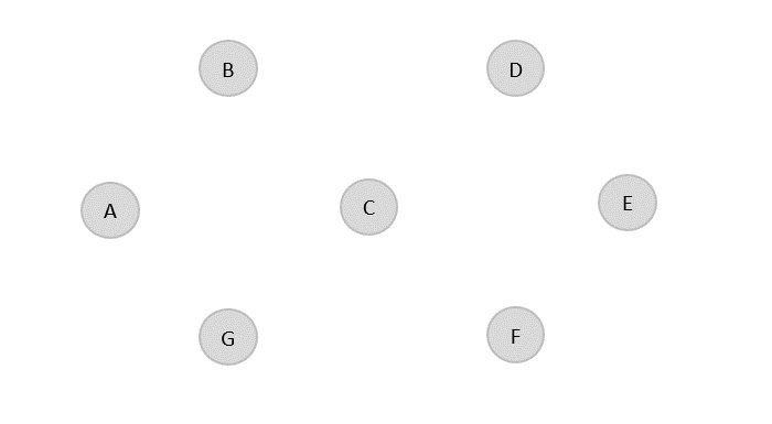
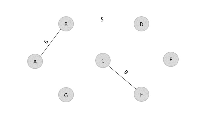
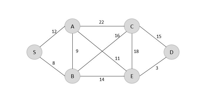
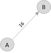
Initial Set

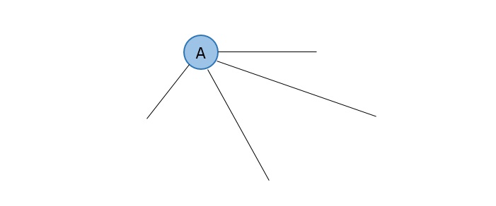
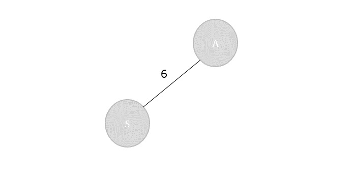
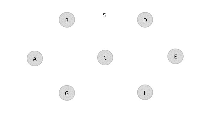
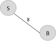
Step 1
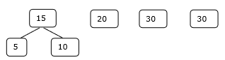
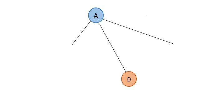
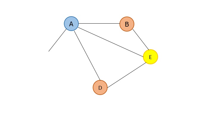
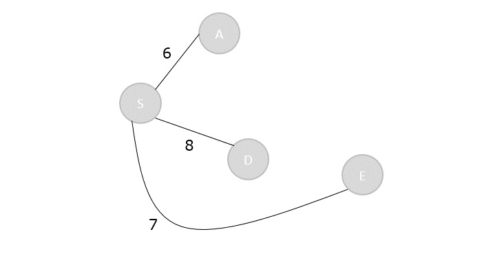
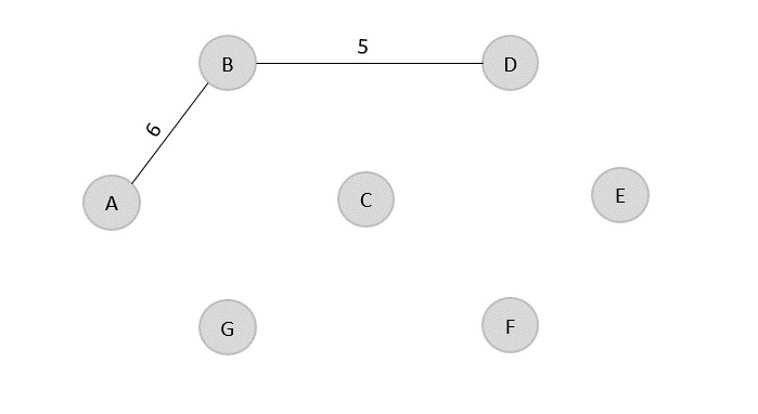
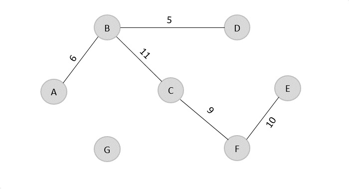
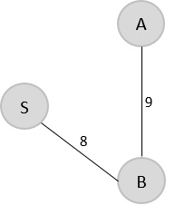
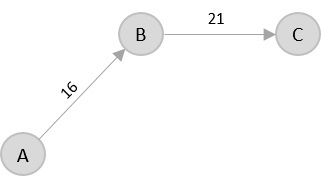
Step 2
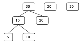
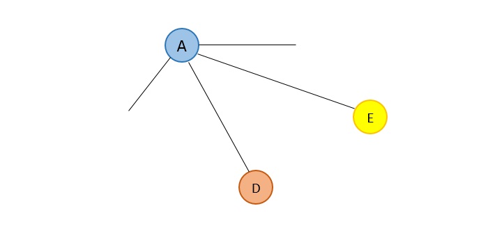
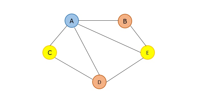
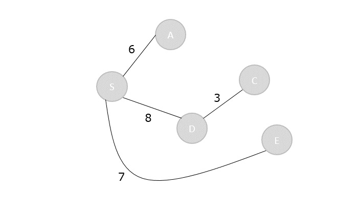
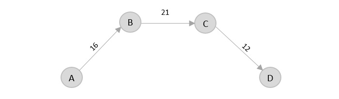
Step 3
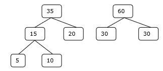
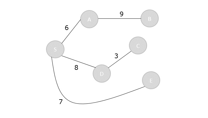
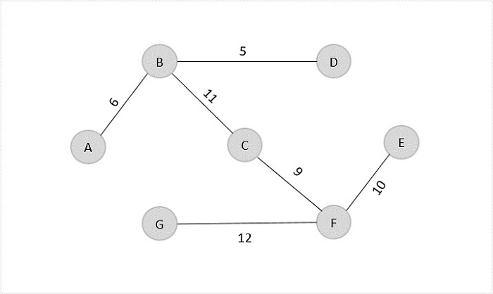
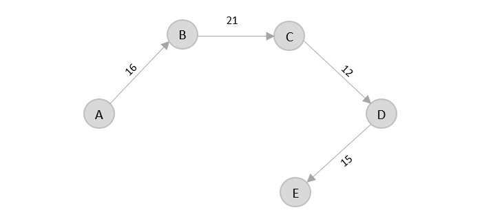
Step 4
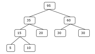
Hence, the solution takes 15 + 35 + 60 + 95 = 205 number of comparisons.
Example
Following are the implementations of the above approach in various programming languages −
#include <stdio.h>#include <stdlib.h>intoptimalMerge(int files[],int n){// Sort the files in ascending orderfor(int i =0; i < n -1; i++){for(int j =0; j < n - i -1; j++){if(files[j]> files[j +1]){int temp = files[j];
                files[j]= files[j +1];
                files[j +1]= temp;}}}int cost =0;while(n >1){// Merge the smallest two filesint mergedFileSize = files[0]+ files[1];
        cost += mergedFileSize;// Replace the first file with the merged file size
        files[0]= mergedFileSize;// Shift the remaining files to the leftfor(int i =1; i < n -1; i++){
            files[i]= files[i +1];}
        n--;// Reduce the number of files// Sort the files againfor(int i =0; i < n -1; i++){for(int j =0; j < n - i -1; j++){if(files[j]> files[j +1]){int temp = files[j];
                    files[j]= files[j +1];
                    files[j +1]= temp;}}}}return cost;}intmain(){int files[]={5,10,20,30,30};int n =sizeof(files)/sizeof(files[0]);int minCost =optimalMerge(files, n);printf("Minimum cost of merging is: %d Comparisons\n", minCost);return0;}
Output
Minimum cost of merging is: 205 Comparisons