Category: Graph Data Structure

  • Maxflow Mincut Theorem

    Let’s talk about Maxflow and Mincut. These are like two sides of the same coin when dealing with network flow problems. If you ever wondered how stuff moves through a network, whether its water in pipes, cars on roads, or data in a network, then youre already thinking in terms of max flow and min cut.

    What is Maxflow?

    Maxflow (Maximum Flow) is all about figuring out the most stuff (data, water, traffic) that can move from one point (source) to another (sink) in a network without breaking any capacity limits. Imagine a bunch of pipes carrying water, and you want to know the maximum amount of water that can flow through the system without overflowing.

    What is Mincut?

    Mincut (Minimum Cut) is kind of the opposite. Its about finding the weakest link in the network that, if cut, would completely stop the flow from the source to the sink. Think of it like identifying the narrowest point in a road system where a traffic jam would completely block all movement.

    Maxflow and Mincut Theorem

    Heres something cool: The Maxflow-Mincut Theorem says that the maximum flow in a network is equal to the total capacity of the smallest set of edges that, if removed, would stop the flow completely. This means if you

    These concepts arent just theoretical; they are used in real life all the time:

    • Traffic Management: Figuring out the best way to manage congestion in roads.
    • Computer Networks: Making sure data packets travel efficiently.
    • Airline Scheduling: Ensuring flights are assigned to routes in the best way possible.
    • Water Distribution: Managing water flow in pipelines to avoid shortages.
    • Project Management: Finding the critical path in workflows to improve efficiency.

    Example to Understand Maxflow

    Imagine a city with roads connecting different areas. If you want to get the max number of cars from the start point to the endpoint, thats maxflow. Now, let’s write code.

    Maxflow using Ford-Fulkerson Algorithm

    Steps to find the maxflow in a graph using the Ford-Fulkerson Algorithm:

    1. Start with the initial flow as 0.
    2. While there is an augmenting path from source to sink:
        a. Find the path with the minimum capacity.
        b. Increase the flow along the path.
    3. The maximum flow is the sum of all flows along the augmenting paths.
    

    Here’s the code to find the maxflow in a graph using the Ford-Fulkerson Algorithm:

    CC++JavaPython

    #include <stdio.h>#include <string.h>#include <limits.h>#define V 6  // Number of vertices// Function to perform DFS and find an augmenting pathintdfs(int rGraph[V][V],int s,int t,int parent[]){int visited[V];memset(visited,0,sizeof(visited));int stack[V], top =-1;
       stack[++top]= s;
       visited[s]=1;while(top >=0){int u = stack[top--];for(int v =0; v < V; v++){if(!visited[v]&& rGraph[u][v]>0){
                stack[++top]= v;
                visited[v]=1;
                parent[v]= u;if(v == t){return1;}}}}return0;}// Ford-Fulkerson algorithm to find the max-flowintfordFulkerson(int graph[V][V],int source,int sink){int rGraph[V][V];// Residual graphfor(int i =0; i < V; i++){for(int j =0; j < V; j++){
             rGraph[i][j]= graph[i][j];}}int parent[V];int maxFlow =0;// Augment the flow while there is an augmenting pathwhile(dfs(rGraph, source, sink, parent)){int pathFlow = INT_MAX;for(int v = sink; v != source; v = parent[v]){int u = parent[v];
             pathFlow =(pathFlow < rGraph[u][v])? pathFlow : rGraph[u][v];}
          maxFlow += pathFlow;// Update the residual graphfor(int v = sink; v != source; v = parent[v]){int u = parent[v];
             rGraph[u][v]-= pathFlow;
             rGraph[v][u]+= pathFlow;}}return maxFlow;}intmain(){// Example graphint graph[V][V]={{0,16,13,0,0,0},{0,0,10,12,0,0},{0,4,0,0,14,0},{0,0,9,0,0,20},{0,0,0,7,0,4},{0,0,0,0,0,0}};int source =0, sink =5;printf("Maximum flow: %d\n",fordFulkerson(graph, source, sink));return0;}

    Output

    Following is the output of the above code:

    Maximum flow: 23
    

    Example to Understand Mincut

    We already know what mincut is, let’s code to find the mincut in a graph using the Ford-Fulkerson Algorithm:

    Mincut using Ford-Fulkerson Algorithm

    Steps to find the mincut in a graph using the Ford-Fulkerson Algorithm:

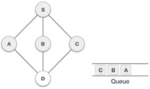
    Initialize the graph and residual graph, and set up the parent[] array to track paths.
    Perform BFS to find an augmenting path from source to sink in the residual graph.
    Update residual graph by reducing the flow along the found path and adding reverse flow.
    Repeat BFS until no augmenting path is found.
    Perform DFS to find all reachable vertices from the source in the residual graph.
    Print the edges that go from a reachable vertex to a non-reachable vertex, which form the minimum cut.
    

    Now, let’s see how to find the mincut in a graph using the Ford-Fulkerson Algorithm:

    CC++JavaPython

    #include <stdio.h>#include <string.h>#include <limits.h>#include <stdbool.h>#define V 6// Simple queue structure for BFStypedefstruct{int items[V];int front, rear;} Queue;voidinitQueue(Queue* q){
       q->front =-1;
       q->rear =-1;}intisEmpty(Queue* q){return q->front ==-1;}voidenqueue(Queue* q,int value){if(q->rear == V -1)return;// Queue overflowif(q->front ==-1)
          q->front =0;
       q->items[++(q->rear)]= value;}intdequeue(Queue* q){if(isEmpty(q))return-1;// Queue underflowint item = q->items[q->front];if(q->front == q->rear)
          q->front = q->rear =-1;else
          q->front++;return item;}intbfs(int rGraph[V][V],int s,int t,int parent[]){
       bool visited[V];memset(visited,0,sizeof(visited));
    
       Queue q;initQueue(&q);enqueue(&q, s);
       visited[s]=1;
       parent[s]=-1;while(!isEmpty(&q)){int u =dequeue(&q);for(int v =0; v < V; v++){if(!visited[v]&& rGraph[u][v]>0){enqueue(&q, v);
                parent[v]= u;
                visited[v]=1;}}}return(visited[t]==1);}voiddfs(int rGraph[V][V],int s, bool visited[]){
       visited[s]=1;for(int i =0; i < V; i++){if(rGraph[s][i]&&!visited[i])dfs(rGraph, i, visited);}}voidminCut(int graph[V][V],int s,int t){int u, v;int rGraph[V][V];for(u =0; u < V; u++){for(v =0; v < V; v++){
             rGraph[u][v]= graph[u][v];}}int parent[V];while(bfs(rGraph, s, t, parent)){int path_flow = INT_MAX;for(v = t; v != s; v = parent[v]){
             u = parent[v];
             path_flow =(path_flow < rGraph[u][v])? path_flow : rGraph[u][v];}for(v = t; v != s; v = parent[v]){
             u = parent[v];
             rGraph[u][v]-= path_flow;
             rGraph[v][u]+= path_flow;}}
    
       bool visited[V];memset(visited,0,sizeof(visited));dfs(rGraph, s, visited);for(int i =0; i < V; i++){for(int j =0; j < V; j++){if(visited[i]&&!visited[j]&& graph[i][j]){printf("%d - %d\n", i, j);}}}}intmain(){int graph[V][V]={{0,10,0,10,0,0},{0,0,5,0,0,0},{0,0,0,0,10,0},{0,0,0,0,0,20},{0,0,0,0,0,10},{0,0,0,0,0,0}};printf("Minimum Cut Edges: \n");minCut(graph,0,5);return0;}

    Output

    Following is the output of the above code:

    Minimum Cut Edges:
    0 - 3
    1 - 2
    

    Conclusion

    Maxflow helps us figure out how much we can push through a system, while Mincut tells us where the weakest spots are. Both are super useful in real-life applications, from networks to transportation and beyond. Learning these concepts can help solve big optimization problems in different fields.

  • Edmond’s Blossom Algorithm

    The Edmonds Blossom Algorithm is used to find the maximum matchings in general graphs. It extends the Blossom Algorithm, which is designed for bipartite graphs. The Edmonds Blossom Algorithm works with any graph, making it a versatile tool for solving matching problems.

    Why Edmonds Blossom Algorithm?

    The Edmonds Blossom Algorithm is a smart way to find the largest possible matchings in general graphs. It’s an extension of the Blossom Algorithm, which was originally created to work with bipartite graphs.

    By building on the Blossom Algorithm, the Edmonds Blossom Algorithm can also work with more complicated graphs, making it more versatile and efficient at finding maximum matchings with fewer steps.

    Edmonds Blossom Algorithm Example

    Consider a simple graph with vertices and edges. Our goal is to find a maximum matching using the Edmonds Blossom Algorithm. The graph is shown below:

       A----B----D
       / \ /     |
      C---E      F   
    

    matching is a set of edges where no two edges share a common vertex. A maximum matching contains the maximum number of edges possible.

    Edmonds Blossom Algorithm Steps

    The Edmonds Blossom Algorithm finds augmenting paths in the graph to increase the matching size. Here are the steps:

    1. Find an augmenting path, which is a path from a free vertex to another free vertex that alternates between matched and unmatched edges.
    2. If an augmenting path is found, update the matching by flipping the edges along the path, increasing the matching size by one.
    3. If no augmenting path is found, the current matching is maximum, and the algorithm stops.
    4. Repeat steps 1-3 until no more augmenting paths are found.
    

    Following these steps, the Edmonds Blossom Algorithm efficiently finds a maximum matching in a general graph.

    Code for Edmonds Blossom Algorithm

    Here’s an example code snippet for the Edmonds Blossom Algorithm in C, C++, Java, and Python:

    CC++JavaPython

    #include <stdio.h>#include <stdlib.h>#include <string.h>#define MAX_VERTICES 6#define MAX_EDGES 6int adj[MAX_VERTICES][MAX_VERTICES]={{0,1,1,0,0,0},{1,0,0,1,1,0},{1,0,0,0,1,0},{0,1,0,0,0,1},{0,1,1,0,0,0},{0,0,0,1,0,0}};int match[MAX_VERTICES];int visited[MAX_VERTICES];intfind_augmenting_path(int u){for(int v =0; v < MAX_VERTICES; v++){if(adj[u][v]&&!visited[v]){
             visited[v]=1;if(match[v]==-1||find_augmenting_path(match[v])){
                match[v]= u;return1;}}}}intedmonds_blossom_algorithm(){memset(match,-1,sizeof(match));int max_matching =0;for(int u =0; u < MAX_VERTICES; u++){memset(visited,0,sizeof(visited));if(find_augmenting_path(u)){
             max_matching++;}}return max_matching;}intmain(){int max_matching =edmonds_blossom_algorithm();printf("Maximum Matching: %d\n", max_matching);return0;}

    Output

    Following is the output of the above code:

    Maximum Matching: 6
    

    Applications of Edmonds Blossom Algorithm

    The Edmonds Blossom Algorithm is used in various applications, including:

    • Matching problems: Finding maximum matchings in graphs for scheduling, resource allocation, and network design.
    • Graph theory: Studying graph properties and their applications in computer science and other fields.
    • Combinatorial optimization: Solving problems that involve finding the best solution from a finite set of possibilities.

    Conclusion

    In this chapter, we discussed the Edmonds Blossom Algorithm, why it’s useful and steps to implement it. We have also provided example code snippets in CC++Java, and Python to demonstrate how the Edmonds Blossom Algorithm works. And we explored application of the Edmonds Blossom Algorithm.

  • Flow Networks

    Flow networks are a special kind of graph that are used for representing the flow of data or resources from one point to another. They are used in a variety of applications, including transportation networks, communication networks, and computer networks. In this chapter, we will discuss the basic concepts of flow networks and how they are used in data structures.

    What is a Flow Network?

    flow network is a directed graph in which each edge has a capacity and a flow. The capacity of an edge represents the maximum amount of flow that can pass through it, while the flow of an edge represents the actual amount of flow passing through it. The flow of an edge must be less than or equal to its capacity.

    Flow networks are used to model the flow of data or resources from a source to a sink. The source is the starting point of the flow, while the sink is the ending point. The goal of a flow network is to maximize the flow from the source to the sink while respecting the capacities of the edges.

    Flow Network Example

    Let’s consider a simple flow network with a source, a sink, and some intermediate nodes. The edges of the flow network have capacities and flows as shown below:

            10(5)
        A --------> B
        |           |
       5(3)        8(6)
        |           |
        v           v
        C --------> D
            7(4)    | 6(4)
                    v
                    E
                    | 4(4)
                    v
                    F


    The flow network represents the flow of data from the source A to the sink F. The goal is to maximize the flow from A to F while respecting the capacities of the edges. In this example, the maximum flow from A to F is 10, which is achieved by sending 5 units of flow along edge AB, 3 units along edge AC, 6 units along edge BD, 4 units along edge CE, and 4 units along edge EF.

    • Edge AB: Capacity = 10, Flow = 5
    • Edge AC: Capacity = 5, Flow = 3
    • Edge BD: Capacity = 8, Flow = 6
    • Edge CE: Capacity = 7, Flow = 4
    • Edge DE: Capacity = 6, Flow = 4
    • Edge EF: Capacity = 4, Flow = 4

    Flow Network Algorithms

    There are several algorithms that can be used to find the maximum flow in a flow network. Some of the most common algorithms include:

    1. Ford-Fulkerson Algorithm
    2. Edmonds-Karp Algorithm
    3. Dinic’s Algorithm
    4. Push-Relabel Algorithm

    These algorithms use different techniques to find the maximum flow in a flow network. They are based on the concept of augmenting paths, which are paths from the source to the sink that can carry additional flow. By finding augmenting paths and increasing the flow along them.

    Ford-Fulkerson Algorithm to Find Maximum Flow

    Let’s take a look at the Ford-Fulkerson algorithm, which is one of the most popular algorithms for finding the maximum flow in a flow network. The algorithm works by finding augmenting paths from the source to the sink and increasing the flow along these paths.

    The steps of the Ford-Fulkerson algorithm are as follows:

    1. Initialize the flow of each edge to 0.
    2. While there is an augmenting path from the source to the sink:
        a. Find an augmenting path using a depth-first search or breadth-first search.
        b. Determine the maximum flow that can be sent along the augmenting path.
        c. Increase the flow along the augmenting path by the maximum flow.
    3. Return the maximum flow.
    

    By following these steps, the Ford-Fulkerson algorithm can find the maximum flow in a flow network. The algorithm terminates when there are no more augmenting paths from the source to the sink.

    Code for Ford-Fulkerson Algorithm

    Here’s an example code snippet for the Ford-Fulkerson algorithm in C, C++, Java, and Python:

    CC++JavaPython

    #include <stdio.h>#include <limits.h>#include <stdbool.h>#include <string.h>#define V 6
    
    bool bfs(int rGraph[V][V],int s,int t,int parent[]){
       bool visited[V];memset(visited,0,sizeof(visited));int queue[V];int front =0, rear =0;
       queue[rear++]= s;
       visited[s]= true;
       parent[s]=-1;while(front != rear){int u = queue[front++];for(int v =0; v < V; v++){if(!visited[v]&& rGraph[u][v]>0){
                queue[rear++]= v;
                parent[v]= u;
                visited[v]= true;}}}return visited[t];}intfordFulkerson(int graph[V][V],int s,int t){int u, v;int rGraph[V][V];for(u =0; u < V; u++)for(v =0; v < V; v++)
             rGraph[u][v]= graph[u][v];int parent[V];int max_flow =0;while(bfs(rGraph, s, t, parent)){int path_flow = INT_MAX;for(v = t; v != s; v = parent[v]){
             u = parent[v];
             path_flow = path_flow < rGraph[u][v]? path_flow : rGraph[u][v];}for(v = t; v != s; v = parent[v]){
             u = parent[v];
             rGraph[u][v]-= path_flow;
             rGraph[v][u]+= path_flow;}
    
          max_flow += path_flow;}return max_flow;}intmain(){int graph[V][V]={{0,10,5,0,0,0},{0,0,0,8,0,0},{0,0,0,0,7,0},{0,0,0,0,6,6},{0,0,0,0,0,4},{0,0,0,0,0,0}};printf("The maximum possible flow is %d\n",fordFulkerson(graph,0,5));return0;}

    Output

    Following is the output of the above code:

    The maximum possible flow is 10
    

    Applications of Flow Networks

    Flow networks are used in a variety of applications, including:

    • Transportation networks: Flow networks can be used to model the flow of traffic on roads, railways, and other transportation systems.
    • Communication networks: Flow networks can be used to model the flow of data in computer networks, telecommunication networks, and other communication systems.
    • Supply chain networks: Flow networks can be used to model the flow of goods, materials, and resources in supply chain networks.
    • Fluid networks: Flow networks can be used to model the flow of fluids in pipelines, water distribution systems, and other fluid systems.

    By using flow networks, engineers and researchers can analyze and optimize the flow of data or resources in a wide range of applications. Flow networks are a powerful tool for modeling complex systems and finding efficient solutions to flow-related problems.

    Conclusion

    In this chapter, we discussed the concept of flow networks and how they are used in data structures. We also explored the Ford-Fulkerson algorithm, which is one of the most popular algorithms for finding the maximum flow in a flow network. By understanding flow networks and the algorithms used to analyze them, you can solve a wide range of flow-related problems in various domains.

  • Network Flow Problems

    Network flow problems are all about figuring out how stuff (data, resources, whatever) can move from a start point (source) to an endpoint (sink) in a network. Its like optimizing a traffic system, a data network, or even supply chains. In this article, well talk about what network flow problems are and how we handle them using data structures.

    What are Network Flow Problems?

    So, network flow problems deal with this idea of moving flow from one point to another. We have a network of nodes connected by edges, and each edge has a capacity. The capacity shows how much can actually flow through that edge, and the flow is the amount thats actually moving. The rule is that the flow on an edge can’t be more than its capacity.

    The whole point of these problems is to move as much “stuff” (data, goods, etc.) as we can from the source to the sink. But we have to respect the limits (capacities) of each edge along the way. The goal is to maximize the flow without breaking any edges.

    Network Flow Problem Example

    Imagine we have a simple network with a source node and a sink node. The nodes are connected by edges with certain capacities. We apply the right algorithm to find out how much flow can go from source to sink while respecting the edge capacities. We want to push as much flow through the network as possible.

    Network Flow Problem Algorithms

    To solve these problems, we use a few different algorithms. They help us figure out the max flow in the network. Heres a quick rundown:

    • Ford-Fulkerson Algorithm: This ones pretty basic. It keeps finding augmenting paths and pushing flow through them until it cant anymore.
    • Edmonds-Karp Algorithm: Its a bit faster than Ford-Fulkerson, using BFS to find the shortest augmenting path.
    • Dinic’s Algorithm: A bit more advanced and faster in some cases. It uses a layered approach.
    • Push-Relabel Algorithm: Works by pushing flow around efficiently and adjusting the flow with labels.

    They all work by finding these paths called augmenting pathspaths where we can add more flow. Its like a race to find the best path to push more stuff through until theres no room left to move more.

    Example of Network Flow Problems

    You are given a directed graph representing a network with capacities on edges. The graph has a source node (s) and a sink node (t). The goal is to determine the maximum flow that can be sent from source to sink while respecting the capacity constraints.

        (0)
        /   \
      10     15
      /       \
    (1)---5---(3)  
      \       /
       10    10
        \   /
         (4)
           \
            10
             \
             (5)


    In the above graph, the numbers on the edges represent the capacities. The maximum flow from source (0) to sink (5) is 20.

    Network Flow Problem Code

    Here’s code for above problem in C, C++, Java, and Python:

    CC++JavaPython

    #include <stdio.h>#include <stdlib.h>#include <string.h>#include <limits.h>  #define MAX_VERTICES 6#define min(a, b) ((a) < (b) ? (a) : (b))intbfs(int rGraph[MAX_VERTICES][MAX_VERTICES],int s,int t,int parent[MAX_VERTICES]){int visited[MAX_VERTICES];memset(visited,0,sizeof(visited));
       visited[s]=1;int queue[MAX_VERTICES];int front =0, rear =0;
       queue[rear++]= s;
       parent[s]=-1;while(front != rear){int u = queue[front++];for(int v =0; v < MAX_VERTICES; v++){if(!visited[v]&& rGraph[u][v]>0){
                queue[rear++]= v;
                parent[v]= u;
                visited[v]=1;if(v == t){return1;}}}}return0;// No more augmenting path}intford_fulkerson(int graph[MAX_VERTICES][MAX_VERTICES],int s,int t){int u, v;int rGraph[MAX_VERTICES][MAX_VERTICES];for(u =0; u < MAX_VERTICES; u++)for(v =0; v < MAX_VERTICES; v++)
             rGraph[u][v]= graph[u][v];int parent[MAX_VERTICES];int max_flow =0;while(bfs(rGraph, s, t, parent)){int path_flow = INT_MAX;for(v = t; v != s; v = parent[v]){
             u = parent[v];
             path_flow =min(path_flow, rGraph[u][v]);}for(v = t; v != s; v = parent[v]){
             u = parent[v];
             rGraph[u][v]-= path_flow;
             rGraph[v][u]+= path_flow;}
    
          max_flow += path_flow;}return max_flow;}intmain(){int adj[MAX_VERTICES][MAX_VERTICES]={{0,10,15,0,0,0},{0,0,0,5,10,0},{0,0,0,0,0,10},{0,0,0,0,0,5},{0,0,0,0,0,10},{0,0,0,0,0,0}};int source =0;int sink =5;int max_flow =ford_fulkerson(adj, source, sink);printf("Maximum flow from source to sink is %d\n", max_flow);return0;}

    Output

    Following is the output of the above code:

    Maximum flow from source to sink is 20
    

    Applications of Network Flow Problems

    These problems arent just theoretical. They show up everywhere! Here are some areas where we use them:

    • Transportation Networks: Traffic, buses, trainsanything that moves people or goods. We use network flow problems to manage how stuff moves around in these systems.
    • Communication Networks: Data, video calls, web trafficall of that depends on network flow. By solving these problems, we can figure out how to route the data in the most efficient way.
    • Supply Chains: Getting goods and materials from one place to another is a classic flow problem. We use these algorithms to optimize how resources move through a supply chain.
    • Fluid Systems: Think water pipes or oil pipelines. We use network flow problems to manage the flow of liquids or gases in these systems.

    By solving network flow problems, engineers and researchers can tweak and improve systems where resources flow from one place to another. Whether its traffic, data, or anything in between, these problems help optimize flow in the best way possible.

    Conclusion

    In this tutorial, we talked about network flow problems and how they help us figure out the best way to move stuff from one place to another. We use algorithms to find the maximum flow in a network, respecting the capacities of each edge. These problems show up in all sorts of systems, from transportation to communication to supply chains. By solving network flow problems, we can optimize how resources move around in these systems, making them more efficient and effective.

  • What Is an Augmenting Path?

    An augmenting path in a graph is just a way to get from the source to the sink where we can push more flow. In a flow network, the goal is to find these paths and increase the flow along them, ultimately making the total flow as big as possible.

    These paths are essential in finding the maximum flow from the source to the sink in flow networks.

    Augmenting Path Example

    Lets break it down with an example. Imagine we have a simple flow network with a source, a sink, and a few intermediate nodes. Each edge between nodes has a capacity (how much it can carry) and flow (how much is currently flowing). Here’s how it looks:

    In this network, node A is the source and node F is the sink. The capacities and flows of the edges are as follows:

    • Edge AB: Capacity = 10, Flow = 5
    • Edge AC: Capacity = 15, Flow = 10
    • Edge BD: Capacity = 5, Flow = 3
    • Edge BE: Capacity = 10, Flow = 7
    • Edge CF: Capacity = 10, Flow = 8

    This flow network shows how data flows from A to F. The key here is to push as much flow as possible while respecting the capacities of the edges. In this case, the maximum flow from A to F is 15, which is achieved by sending 5 units of flow through edge AB10 units through edge AC, and 5 units through edge CF. But theres still room for improvement by finding augmenting paths to push more flow through!

    Augmenting Path Algorithms

    Now, lets talk about some algorithms that help us find these augmenting paths. There are a few options, and they work in different ways to maximize the flow:

    • Ford-Fulkerson Algorithm: This is a basic and simple approach, but it might not be the fastest.
    • Edmonds-Karp Algorithm: This one is more efficient because it uses BFS to find augmenting paths.
    • Dinic’s Algorithm: A more advanced method that uses a layered approach for better performance.
    • Push-Relabel Algorithm: Instead of finding paths directly, this method pushes excess flow and adjusts labels to optimize the flow.

    Implemention of Augmenting Paths

    Now that we know what augmenting paths are and how they help us increase the flow in a network, lets see how we can implement them in code. Heres a simple example of the Ford-Fulkerson algorithm –

    Algorithm for Augmenting Paths

    1. Create a residual graph with the same capacities as the original graph.
    2. While theres an augmenting path from the source to the sink:
       a. Find the path using a search algorithm (like BFS).
       b. Determine the maximum flow that can be pushed through the path.
       c. Update the residual graph by reducing the capacities of forward edges and increasing the capacities of backward edges.
    3. Return the maximum flow found.
    

    Code for Augmenting Paths

    Heres a simple code snippet that uses the Ford-Fulkerson algorithm to find the maximum flow in a flow network:

    CC++JavaPython

    #include <stdio.h>#include <limits.h>#include <stdbool.h>#define V 6
    
    bool bfs(int rGraph[V][V],int s,int t,int parent[]){
       bool visited[V]={false};int queue[V];int front =0, rear =0;
       queue[rear++]= s;
       visited[s]= true;
       parent[s]=-1;while(front != rear){int u = queue[front++];for(int v =0; v < V; v++){if(!visited[v]&& rGraph[u][v]>0){
                queue[rear++]= v;
                parent[v]= u;
                visited[v]= true;}}}return visited[t];}intfordFulkerson(int graph[V][V],int s,int t){int u, v;int rGraph[V][V];for(u =0; u < V; u++){for(v =0; v < V; v++){
             rGraph[u][v]= graph[u][v];}}int parent[V];int max_flow =0;while(bfs(rGraph, s, t, parent)){int path_flow = INT_MAX;for(v = t; v != s; v = parent[v]){
             u = parent[v];
             path_flow = path_flow < rGraph[u][v]? path_flow : rGraph[u][v];}for(v = t; v != s; v = parent[v]){
             u = parent[v];
             rGraph[u][v]-= path_flow;
             rGraph[v][u]+= path_flow;}
    
          max_flow += path_flow;}return max_flow;}intmain(){int graph[V][V]={{0,10,15,0,0,0},{0,0,0,5,10,0},{0,0,0,0,0,10},{0,0,0,0,0,5},{0,0,0,0,0,10},{0,0,0,0,0,0}};printf("The maximum possible flow is %d\n",fordFulkerson(graph,0,5));return0;}

    Output

    Following is the output of the above code:

    The maximum possible flow is 20
    

    Each of these algorithms helps us find the best paths to push more flow through the network and, eventually, determine the maximum flow possible.

    Real-Life Uses of Augmenting Paths

    Augmenting paths are super useful in many real-world situations, especially when we need to manage the flow of things like datatraffic, or materials. Here are some areas where these concepts come in handy:

    • Transportation Networks: Augmenting paths can be used to model how traffic moves through roadsrailways, and other transport systems. This helps us optimize traffic flow.
    • Communication Networks: In computer and telecom networks, augmenting paths can help manage data flow and figure out the most efficient way to route information.
    • Supply Chain Networks: In supply chains, augmenting paths help track the flow of goods and materials, ensuring smooth movement from suppliers to customers.
    • Fluid Systems: Augmenting paths can also be applied in systems that move liquids or gases, like pipes or water distribution systems, to make sure everything flows as efficiently as possible.

    By using augmenting paths, engineers can better understand how things flow through these systems and find ways to improve them. Whether its transportationcommunicationsupply chains, or fluid systems, these techniques help us optimize how resources move and find the most efficient solutions!

  • Bi-connected Components

    Imagine you have a big network of cities (nodes) connected by roads (edges). Now, if you remove just one city, and the whole network breaks into separate parts, then that city is called an articulation point (or cut vertex).

    So, Bi-connected Components(BCC) are the largest possible parts of a graph(subgraph) where no single node removal can disconnect them.

    For example, consider the following graph:

    Biconnected Components

    The articulation points in the graph are:

    {2}
    {4}
    {6}
    

    The Bi-connected Components (BCCs) in the graph are:

    {0, 1, 2, 3}
    {2, 4}
    {4, 5}
    {4, 6}
    {6, 7, 8}
    

    Properties of Bi-connected Components

    Here are some key properties of bi-connected components:

    • Edge: Every edge belongs to exactly one biconnected component.
    • Articulation Points: A node can have multiple biconnected components, but it can be an articulation point for only one of them.
    • Bridge: An edge that, when removed, increases the number of biconnected components.
    • If a graph has no articulation points, the whole graph itself is BCC.

    Algorithm for Finding BCC

    We use DFS(depth first search) to find biconnected components.

    Here’s a simple algorithm to find biconnected components in a graph:

    1. Perform a Depth First Search (DFS) traversal of the graph.
    2. During the DFS traversal, maintain a stack to keep track of the nodes visited.
    3. For each node, keep track of the discovery time and low value.
    4. When visiting a node, push it onto the stack and update the discovery time and low value.
    5. If a back edge is found (i.e., an edge to an already visited node), update the low value of the current node.
    6. If the low value of the current node is less than or equal to the discovery time of the parent node, pop nodes from the stack until the current node is reached.
    7. The popped nodes form a biconnected component.
    

    Let’s say we have this graph

         A
        / \
       B   C
       |   |
       D - E
          / \
         F   G 
    

    The edges are:

    AB, AC, BD, CE, EF, EG, DE
    

    If we remove node E, the graph look like this:

         A
        / \
       B   C
       |   
       D        E
               / \
              F   G
    
    • {A, B, C, D, E}
    • {E, F, G}

    Code for Biconnected Components

    Let’s see the code for finding biconnected components in a above graph:

    CC++JavaPython

    #include <stdio.h>#include <stdlib.h>#include <string.h>#include <stdbool.h>#define MAX 100int time =0;int disc[MAX], low[MAX], parent[MAX];
    bool visited[MAX];typedefstruct{int u, v;} Edge;
    
    Edge stack[MAX];int top =-1;// Mapping indexes to letterschar nodes[]={'A','B','C','D','E','F','G'};voidpush(int u,int v){
       stack[++top].u = u;
       stack[top].v = v;}voidpopUntil(int u,int v){printf("\nBiconnected Component: ");while(top >=0){printf("{%c, %c} ", nodes[stack[top].u], nodes[stack[top].v]);if(stack[top].u == u && stack[top].v == v){
             top--;break;}
          top--;}}voidDFS(int graph[MAX][MAX],int u,int n){
       visited[u]= true;
       disc[u]= low[u]=++time;for(int v =0; v < n; v++){if(graph[u][v]){if(!visited[v]){
                parent[v]= u;push(u, v);DFS(graph, v, n);
    
                low[u]=(low[u]< low[v])? low[u]: low[v];if(low[v]>= disc[u]){popUntil(u, v);}}elseif(v != parent[u]&& disc[v]< disc[u]){
                low[u]=(low[u]< disc[v])? low[u]: disc[v];push(u, v);}}}}voidfindBCC(int graph[MAX][MAX],int n){memset(visited, false,sizeof(visited));memset(parent,-1,sizeof(parent));memset(disc,0,sizeof(disc));memset(low,0,sizeof(low));for(int i =0; i < n; i++){if(!visited[i]){DFS(graph, i, n);}}if(top >=0){printf("\nRemaining Biconnected Component: ");while(top >=0){printf("{%c, %c} ", nodes[stack[top].u], nodes[stack[top].v]);
             top--;}}}intmain(){int n =7;int graph[MAX][MAX]={0};
    
       graph[0][1]= graph[1][0]=1;// A-B
       graph[0][2]= graph[2][0]=1;// A-C
       graph[1][3]= graph[3][1]=1;// B-D
       graph[2][4]= graph[4][2]=1;// C-E
       graph[4][5]= graph[5][4]=1;// E-F
       graph[4][6]= graph[6][4]=1;// E-G
       graph[3][4]= graph[4][3]=1;// D-Eprintf("Biconnected Components are:\n");findBCC(graph, n);return0;}

    Output

    Following is the output of the above code:

    Biconnected Components are:
    
    Biconnected Component: {E, F} 
    Biconnected Component: {E, G} 
    Biconnected Component: {C, A} {E, C} {D, E} {B, D} {A, B} 
    

    Time Complexity of BCC

    • The time complexity of finding biconnected components using the above algorithm is O(V + E), where V is the number of vertices and E is the number of edges in the graph.

    Applications of Biconnected Components

    Biconnected components are used in various applications, such as:

    • Network Reliability: If you want to know the weakest link in a network, BCC helps.
    • Bridges & Roads: Cities connected by roads? Find which roads are critical.
    • Computer Networks: In network design, BCC helps in fault tolerance.
    • File Systems: Used in distributed storage systems to avoid single points of failure.

    Conclusion

    We have learned about biconnected components in a graph. We have seen how to find biconnected components using a simple algorithm. We have also seen the code in C, C++, Java, and Python. Biconnected components are essential in network design, fault tolerance, and distributed systems.

  • Strongly Connected Components

    Strongly Connected Components (SCCs) are specific sub-graphs in a directed graph where every node can reach every other node within that sub-graph. In simple terms, SCCs are clusters of nodes that are tightly connected but are separate from other parts of the graph. Understanding SCCs is important, as they help in detecting cycles and studying network structures.

    A directed graph is said to be strongly connected if every node can reach every other node directly or indirectly. However, in larger graphs, we may have multiple strongly connected parts that are not connected to each other. These independent sections are called strongly connected components.

    For example, consider a directed graph with nodes A, B, C, D, and E. If A can reach B and B can reach A, but C, D, and E form a separate cluster where they can all reach each other but not A or B, then there are two SCCs in the graph: {A, B} and {C, D, E}.

    Strongly Connected Components Algorithm

    There are two popular algorithms to find strongly connected components in a graph:

    • Kosaraju’s Algorithm
    • Tarjan’s Algorithm

    Kosaraju’s Algorithm

    Kosaraju’s Algorithm is a two-pass algorithm that finds strongly connected components in a directed graph. Here’s how it works:

    • First Pass: Perform a Depth First Search (DFS) on the graph and store the order of nodes based on their finishing times.
    • Second Pass: Reverse the graph and perform another DFS on the nodes in the order of their finishing times from the first pass. This will give us the strongly connected components.

    Kosaraju’s Algorithm Example

    Let’s consider a directed graph with nodes A, B, C, D, and E, and the following edges:

       A -> B
       B -> C
       C -> A
       C -> D
       D -> E
       E -> D
    

    Using Kosaraju’s Algorithm, we can find the strongly connected components in the graph:

    • First Pass: The finishing times of the nodes are E, D, C, B, A.
    • Second Pass: The strongly connected components are {A, B, C} and {D, E}.

    Code for Kosaraju’s Algorithm

    Here’s an example code snippet for Kosaraju’s Algorithm in C, C++, Java, and Python:

    CC++JavaPython

    #include <stdio.h>#include <stdlib.h>#include <string.h>#define MAX_VERTICES 5// Graph adjacency matrixint adj[MAX_VERTICES][MAX_VERTICES]={{0,1,0,0,0},{0,0,1,0,0},{1,0,0,1,0},{0,0,0,0,1},{0,0,0,1,0}};int visited[MAX_VERTICES]={0};int finishing_time[MAX_VERTICES];int finish_index =0;// Mapping index to letters (A-E)char map[MAX_VERTICES]={'A','B','C','D','E'};voidDFS(int vertex,int print){
       visited[vertex]=1;if(print)printf("%c ", map[vertex]);// Print vertex if it's in SCC traversalfor(int v =0; v < MAX_VERTICES; v++){if(adj[vertex][v]&&!visited[v]){DFS(v, print);}}if(!print) finishing_time[finish_index++]= vertex;// Store finishing time if not printing SCC}voidreverse_graph(){int temp[MAX_VERTICES][MAX_VERTICES];for(int i =0; i < MAX_VERTICES; i++){for(int j =0; j < MAX_VERTICES; j++){
             temp[i][j]= adj[i][j];}}// Transpose the graphfor(int i =0; i < MAX_VERTICES; i++){for(int j =0; j < MAX_VERTICES; j++){
             adj[i][j]= temp[j][i];}}}voidfind_scc(){// Step 1: Compute finishing times in the original graphfor(int v =0; v < MAX_VERTICES; v++){if(!visited[v]){DFS(v,0);// First pass DFS (store finish times)}}// Step 2: Reverse the graphreverse_graph();// Step 3: Second DFS based on decreasing finishing timesmemset(visited,0,sizeof(visited));// Reset visited arrayprintf("Strongly Connected Components:\n");for(int i = MAX_VERTICES -1; i >=0; i--){int vertex = finishing_time[i];if(!visited[vertex]){printf("SCC: ");DFS(vertex,1);// Second pass DFS (print SCC)printf("\n");}}}intmain(){find_scc();return0;}

    Output

    Following is the output of the above code:

    Strongly Connected Components:
    SCC: A C B
    SCC: D E
    

    Tarjan’s Algorithm

    Tarjan’s Algorithm is another popular algorithm to find strongly connected components in a directed graph. It uses Depth First Search (DFS) to traverse the graph and identify SCCs. Here’s how it works:

    • Initialize a stack to keep track of visited nodes and their order of traversal.
    • Perform a DFS traversal of the graph, assigning a unique ID to each node and keeping track of the lowest ID reachable from that node.
    • Nodes with the same ID and low-link value form a strongly connected component.

    Tarjan’s Algorithm Example

    Consider the same directed graph with nodes A, B, C, D, and E, and the following edges:

       A -> B
       B -> C
       C -> A
       C -> D
       D -> E
       E -> D
    

    Using Tarjan’s Algorithm, we can find the strongly connected components in the graph:

    • The strongly connected components are {A, B, C} and {D, E}.

    Code for Tarjan’s Algorithm

    Here’s an example code snippet for Tarjan’s Algorithm in C, C++, Java, and Python:

    CC++JavaPython

    #include <stdio.h>#include <stdlib.h>#include <string.h>#define MAX_VERTICES 5// Graph adjacency matrixint adj[MAX_VERTICES][MAX_VERTICES]={{0,1,0,0,0},{0,0,1,0,0},{1,0,0,1,0},{0,0,0,0,1},{0,0,0,1,0}};int visited[MAX_VERTICES]={0};int stack[MAX_VERTICES];int stack_index =0;int ids[MAX_VERTICES];int low[MAX_VERTICES];int id =0;// Mapping index to letters (A-E)char map[MAX_VERTICES]={'A','B','C','D','E'};int map_index =0;voidDFS(int vertex){
       stack[stack_index++]= vertex;
       visited[vertex]=1;
       ids[vertex]= low[vertex]= id++;for(int v =0; v < MAX_VERTICES; v++){if(adj[vertex][v]){if(!visited[v]){DFS(v);}if(ids[v]!=-1){
                low[vertex]= low[vertex]0){int node = stack[--stack_index];
             low[node]= ids[vertex];printf("%c ", map[node]);if(node == vertex)break;}printf("\n");}}voidfind_scc(){memset(ids,-1,sizeof(ids));memset(low,-1,sizeof(low));for(int v =0; v < MAX_VERTICES; v++){if(!visited[v]){DFS(v);}}}intmain(){find_scc();return0;}

    Output

    Following is the output of the above code:

    SCC: E D
    SCC: C B A
    

    Applications of Strongly Connected Components

    Following are some common applications of Strongly Connected Components:

    • Network Analysis: SCCs help in understanding the structure and connectivity of networks, such as social networks, transportation networks, and communication networks.
    • Graph Algorithms: SCCs are used in various graph algorithms, such as cycle detection, pathfinding, and network flow optimization.
    • Software Engineering: SCCs are useful in software engineering for dependency analysis, module identification, and code refactoring.

    Conclusion

    Understanding Strongly Connected Components is essential for analyzing the connectivity and structure of directed graphs. Algorithms like Kosaraju’s Algorithm and Tarjan’s Algorithm provide efficient ways to identify SCCs in graphs, enabling various applications in network analysis, graph algorithms, and software engineering.

  • Topological Sorting in Graph Data Structure

    Topological sorting is a way of arranging the nodes of a Directed Acyclic Graph (DAG) in a line, making sure that for every directed edge from u to v, node u comes before v. If the graph has cycles, topological sorting isn’t possible.

    In topological sorting, if theres an edge from u to vu should come before v in the order. Its different from DFS, where we visit a node and then explore its neighbors. In topological sorting, a node should be printed before any of its connected nodes.

    Now, lets understand Directed Acyclic Graphs (DAGs). A directed graph has edges that go from one node to another in a specific direction. It is called acyclic if there are no cyclesmeaning theres no way to start from a node and return to it by following edges.

    Topological sorting only works for DAGs. If theres a cycle in the graph, we cant arrange the nodes in a proper order because some nodes will keep pointing back, making a valid linear order impossible.

    Topological Sort

    Topological Sort Algorithm

    Topological sorting can be done using Depth First Search (DFS) algorithm. The algorithm follows the following steps:

    Algorithm

    Following are the steps to perform topological sorting using DFS:

    • Call the DFS function for a vertex u.
    • In the DFS function, mark the vertex u as visited.
    • For every adjacent vertex v of u, if v is not visited, then call the DFS function for vertex v.
    • After visiting all the adjacent vertices of vertex u, add the vertex u to the topological order list.

    After performing the above steps for all the vertices, the topological order list will have the vertices in topological order.

    Code for Topological Sort

    Let’s see the code for topological sorting using Depth First Search (DFS) algorithm:

    CC++JavaPython

    #include <stdio.h>#define MAX_VERTICES 6int adj[MAX_VERTICES][MAX_VERTICES]={{0,1,1,0,0,0},{0,0,0,1,1,0},{0,0,0,0,1,0},{0,0,0,0,0,1},{0,0,0,0,0,1},{0,0,0,0,0,0}};int visited[MAX_VERTICES]={0};int topological_order[MAX_VERTICES];int order_index = MAX_VERTICES -1;voidDFS(int vertex){
       visited[vertex]=1;for(int v =0; v < MAX_VERTICES; v++){if(adj[vertex][v]&&!visited[v]){DFS(v);}}
       topological_order[order_index--]= vertex;}voidtopological_sort(){for(int v =0; v < MAX_VERTICES; v++){if(!visited[v]){DFS(v);}}}voidprint_topological_order(){printf("Topological Order: ");for(int i =0; i < MAX_VERTICES; i++){printf("%d ", topological_order[i]);}printf("\n");}intmain(){topological_sort();print_topological_order();return0;}

    Output

    Following is the output of the above code:

    Topological Order: 0 2 1 3 4 5
    

    Time Complexity of Topological Sort

    When using Depth First Search (DFS) for topological sorting, the time complexity is O(V + E), where V is the number of vertices and E is the number of edges in the graph. This is because we visit each node once and explore all its edges.

    Applications of Topological Sort

    Topological sorting has many applications in various fields. Some of the applications of topological sort are:

    • Task Scheduling: Used to schedule tasks based on dependencies. Each task is a node, and dependencies are edges. This ensures tasks are executed in the correct order.
    • Course Prerequisites: Helps in deciding the order of taking courses. Courses are nodes, and prerequisites are edges, ensuring prerequisites are completed first.
    • Build Systems: Used in software build processes to determine the correct sequence for compiling files based on dependencies.
    • Network Routing: Helps in routing packets through a network by determining the correct order of processing based on connections between routers.
  • Spanning Tree

    What is Spanning Tree?

    A spanning tree is a subset of Graph G, which has all the vertices covered with minimum possible number of edges. Hence, a spanning tree does not have cycles and it cannot be disconnected..

    By this definition, we can draw a conclusion that every connected and undirected Graph G has at least one spanning tree. A disconnected graph does not have any spanning tree, as it cannot be spanned to all its vertices.

    Spanning Trees

    We found three spanning trees off one complete graph. A complete undirected graph can have maximum nn-2 number of spanning trees, where n is the number of nodes. In the above addressed example, n is 3, hence 33−2 = 3 spanning trees are possible.

    General Properties of Spanning Tree

    We now understand that one graph can have more than one spanning tree. Following are a few properties of the spanning tree connected to graph G −

    • A connected graph G can have more than one spanning tree.
    • All possible spanning trees of graph G, have the same number of edges and vertices.
    • The spanning tree does not have any cycle (loops).
    • Removing one edge from the spanning tree will make the graph disconnected, i.e. the spanning tree is minimally connected.
    • Adding one edge to the spanning tree will create a circuit or loop, i.e. the spanning tree is maximally acyclic.

    Mathematical Properties of Spanning Tree

    • Spanning tree has n-1 edges, where n is the number of nodes (vertices).
    • From a complete graph, by removing maximum e – n &plus; 1 edges, we can construct a spanning tree.
    • A complete graph can have maximum nn-2 number of spanning trees.

    Thus, we can conclude that spanning trees are a subset of connected Graph G and disconnected graphs do not have spanning tree.

    Application of Spanning Tree

    Spanning tree is basically used to find a minimum path to connect all nodes in a graph. Common application of spanning trees are −

    • Civil Network Planning
    • Computer Network Routing Protocol
    • Cluster Analysis

    Let us understand this through a small example. Consider, city network as a huge graph and now plans to deploy telephone lines in such a way that in minimum lines we can connect to all city nodes. This is where the spanning tree comes into picture.

    Minimum Spanning Tree (MST)

    In a weighted graph, a minimum spanning tree is a spanning tree that has minimum weight than all other spanning trees of the same graph. In real-world situations, this weight can be measured as distance, congestion, traffic load or any arbitrary value denoted to the edges.

    Minimum Spanning-Tree Algorithm

    We shall learn about two most important spanning tree algorithms here −

    • Kruskal’s Algorithm
    • Prim’s Algorithm

    These two algorithms are Greedy algorithms.

  • Breadth First Search (BFS) Algorithm

    Breadth First Search (BFS) Algorithm

    Breadth First Search (BFS) algorithm traverses a graph in a breadthward motion to search a graph data structure for a node that meets a set of criteria. It uses a queue to remember the next vertex to start a search, when a dead end occurs in any iteration.

    Breadth First Search (BFS) algorithm starts at the tree root and explores all nodes at the present depth prior to moving on to the nodes at the next depth level.

    Breadth First Traversal

    As in the example given above, BFS algorithm traverses from A to B to E to F first then to C and G lastly to D. It employs the following rules.

    • Rule 1 − Visit the adjacent unvisited vertex. Mark it as visited. Display it. Insert it in a queue.
    • Rule 2 − If no adjacent vertex is found, remove the first vertex from the queue.
    • Rule 3 − Repeat Rule 1 and Rule 2 until the queue is empty.
    StepTraversalDescription
    1Breadth First Search Step OneInitialize the queue.
    2Breadth First Search Step TwoWe start from visiting S (starting node), and mark it as visited.
    3Breadth First Search Step ThreeWe then see an unvisited adjacent node from S. In this example, we have three nodes but alphabetically we choose A, mark it as visited and enqueue it.
    4Breadth First Search Step FourNext, the unvisited adjacent node from S is B. We mark it as visited and enqueue it.
    5Breadth First Search Step FiveNext, the unvisited adjacent node from S is C. We mark it as visited and enqueue it.
    6Breadth First Search Step SixNow, S is left with no unvisited adjacent nodes. So, we dequeue and find A.
    7Breadth First Search Step SevenFrom A we have D as unvisited adjacent node. We mark it as visited and enqueue it.

    At this stage, we are left with no unmarked (unvisited) nodes. But as per the algorithm we keep on dequeuing in order to get all unvisited nodes. When the queue gets emptied, the program is over.

    Example

    Following are the implementations of Breadth First Search (BFS) Algorithm in various programming languages −

    CC++JavaPython

    #include <stdio.h>#include <stdlib.h>#include <stdbool.h>#define MAX 5structVertex{char label;
       bool visited;};//queue variablesint queue[MAX];int rear =-1;int front =0;int queueItemCount =0;//graph variables//array of verticesstructVertex* lstVertices[MAX];//adjacency matrixint adjMatrix[MAX][MAX];//vertex countint vertexCount =0;//queue functionsvoidinsert(int data){
       queue[++rear]= data;
       queueItemCount++;}intremoveData(){
       queueItemCount--;return queue[front++];}
    bool isQueueEmpty(){return queueItemCount ==0;}//graph functions//add vertex to the vertex listvoidaddVertex(char label){structVertex* vertex =(structVertex*)malloc(sizeof(structVertex));
       vertex->label = label;  
       vertex->visited = false;     
       lstVertices[vertexCount++]= vertex;}//add edge to edge arrayvoidaddEdge(int start,int end){
       adjMatrix[start][end]=1;
       adjMatrix[end][start]=1;}//display the vertexvoiddisplayVertex(int vertexIndex){printf("%c ",lstVertices[vertexIndex]->label);}//get the adjacent unvisited vertexintgetAdjUnvisitedVertex(int vertexIndex){int i;for(i =0; i<vertexCount; i++){if(adjMatrix[vertexIndex][i]==1&& lstVertices[i]->visited == false)return i;}return-1;}voidbreadthFirstSearch(){int i;//mark first node as visited
       lstVertices[0]->visited = true;//display the vertexdisplayVertex(0);//insert vertex index in queueinsert(0);int unvisitedVertex;while(!isQueueEmpty()){//get the unvisited vertex of vertex which is at front of the queueint tempVertex =removeData();//no adjacent vertex foundwhile((unvisitedVertex =getAdjUnvisitedVertex(tempVertex))!=-1){    
             lstVertices[unvisitedVertex]->visited = true;displayVertex(unvisitedVertex);insert(unvisitedVertex);}}//queue is empty, search is complete, reset the visited flag        for(i =0;i<vertexCount;i++){
          lstVertices[i]->visited = false;}}intmain(){int i, j;for(i =0; i<MAX; i++){// set adjacency for(j =0; j<MAX; j++)// matrix to 0
             adjMatrix[i][j]=0;}addVertex('S');// 0addVertex('A');// 1addVertex('B');// 2addVertex('C');// 3addVertex('D');// 4addEdge(0,1);// S - AaddEdge(0,2);// S - BaddEdge(0,3);// S - CaddEdge(1,4);// A - DaddEdge(2,4);// B - DaddEdge(3,4);// C - Dprintf("\nBreadth First Search: ");breadthFirstSearch();return0;}

    Output

    Breadth First Search: S A B C D
    

    Click to check C implementation of Breadth First Search (BFS) Algorithm

    Complexity of BFS Algorithm

    Time Complexity

    The time complexity of the BFS algorithm is represented in the form of O(V + E), where V is the number of nodes and E is the number of edges.

    Space Complexity

    The space complexity of the BFS algorithm is O(V).