Category: Dynamic Programming

Travelling salesman problem is the most notorious computational problem. We can use brute-force approach to evaluate every possible tour and select the best one. For n number of vertices in a graph, there are (n1)! number of possibilities. Thus, maintaining a higher complexity.

However, instead of using brute-force, using the dynamic programming approach will obtain the solution in lesser time, though there is no polynomial time algorithm.

Travelling Salesman Dynamic Programming Algorithm

Let us consider a graph G = (V,E), where V is a set of cities and E is a set of weighted edges. An edge e(u, v) represents that vertices u and v are connected. Distance between vertex u and v is d(u, v), which should be non-negative.

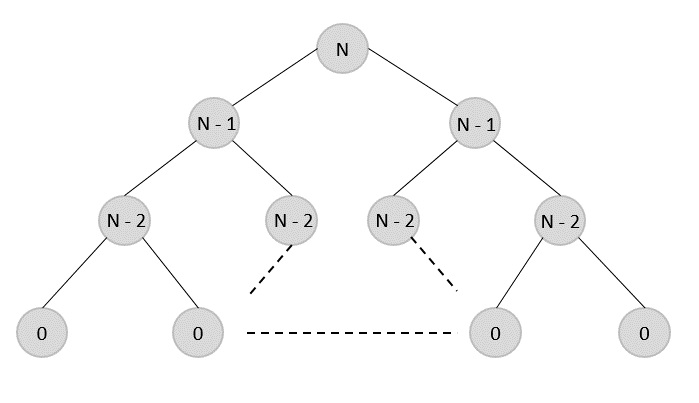
Suppose we have started at city 1 and after visiting some cities now we are in city j. Hence, this is a partial tour. We certainly need to know j, since this will determine which cities are most convenient to visit next. We also need to know all the cities visited so far, so that we don’t repeat any of them. Hence, this is an appropriate sub-problem.

For a subset of cities S ϵ {1,2,3,…,n} that includes 1, and j ϵ S, let C(S, j) be the length of the shortest path visiting each node in S exactly once, starting at 1 and ending at j.

When |S|> 1 , we define C(S,1)= ∝ since the path cannot start and end at 1.

Now, let express C(S, j) in terms of smaller sub-problems. We need to start at 1 and end at j. We should select the next city in such a way that

C(S,j)=minC(S−{j},i)+d(i,j)whereiϵSandi≠j

Algorithm: Traveling-Salesman-Problem
C ({1}, 1) = 0
for s = 2 to n do
   for all subsets S  {1, 2, 3,  , n} of size s and containing 1
      C (S, 1) = ∞
   for all j  S and j  1
      C (S, j) = min {C (S  {j}, i) + d(i, j) for i  S and i  j}
Return minj C ({1, 2, 3, , n}, j) + d(j, i)

Analysis

There are at the most 2ⁿ.n sub-problems and each one takes linear time to solve. Therefore, the total running time is O(2ⁿ.n²).

Example

In the following example, we will illustrate the steps to solve the travelling salesman problem.

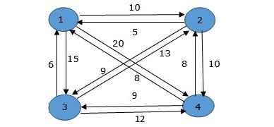
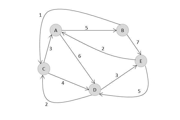
From the above graph, the following table is prepared.

	1	2	3	4
1	0	10	15	20
2	5	0	9	10
3	6	13	0	12
4	8	8	9	0

S = Φ

Cost(2,Φ,1)=d(2,1)=5

Cost(3,Φ,1)=d(3,1)=6

Cost(4,Φ,1)=d(4,1)=8

S = 1

Cost(i,s)=min{Cos(j,s−(j))+d[i,j]}

Cost(2,{3},1)=d[2,3]+Cost(3,Φ,1)=9+6=15

Cost(2,{4},1)=d[2,4]+Cost(4,Φ,1)=10+8=18

Cost(3,{2},1)=d[3,2]+Cost(2,Φ,1)=13+5=18

Cost(3,{4},1)=d[3,4]+Cost(4,Φ,1)=12+8=20

Cost(4,{3},1)=d[4,3]+Cost(3,Φ,1)=9+6=15

Cost(4,{2},1)=d[4,2]+Cost(2,Φ,1)=8+5=13

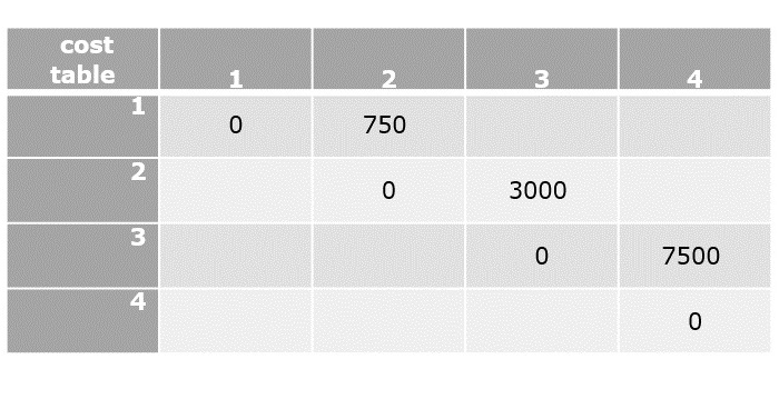
S = 2

Cost(2,{3,4},1)=min{d[2,3]+Cost(3,{4},1)=9+20=29d[2,4]+Cost(4,{3},1)=10+15=25=25

Cost(3,{2,4},1)=min{d[3,2]+Cost(2,{4},1)=13+18=31d[3,4]+Cost(4,{2},1)=12+13=25=25

Cost(4,{2,3},1)=min{d[4,2]+Cost(2,{3},1)=8+15=23d[4,3]+Cost(3,{2},1)=9+18=27=23

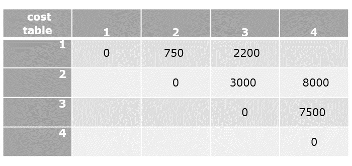
S = 3

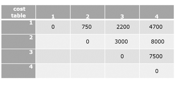
Cost(1,{2,3,4},1)=min⎧⎩⎨⎪⎪d[1,2]+Cost(2,{3,4},1)=10+25=35d[1,3]+Cost(3,{2,4},1)=15+25=40d[1,4]+Cost(4,{2,3},1)=20+23=43=35

The minimum cost path is 35.

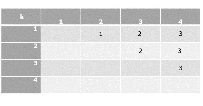
Start from cost {1, {2, 3, 4}, 1}, we get the minimum value for d [1, 2]. When s = 3, select the path from 1 to 2 (cost is 10) then go backwards. When s = 2, we get the minimum value for d [4, 2]. Select the path from 2 to 4 (cost is 10) then go backwards.

When s = 1, we get the minimum value for d [4, 2] but 2 and 4 is already selected. Therefore, we select d [4, 3] (two possible values are 15 for d [2, 3] and d [4, 3], but our last node of the path is 4). Select path 4 to 3 (cost is 9), then go to s = step. We get the minimum value for d [3, 1] (cost is 6).

Implementation

Following are the implementations of the above approach in various programming languages −

CC++JavaPython

#include <stdio.h>#include <limits.h>#define MAX 9999int n =4;int distan[20][20]={{0,22,26,30},{30,0,45,35},{25,45,0,60},{30,35,40,0}};int DP[32][8];intTSP(int mark,int position){int completed_visit =(1<< n)-1;if(mark == completed_visit){return distan[position][0];}if(DP[mark][position]!=-1){return DP[mark][position];}int answer = MAX;for(int city =0; city < n; city++){if((mark &(1<< city))==0){int newAnswer = distan[position][city]+TSP(mark |(1<< city), city);
         answer =(answer < newAnswer)? answer : newAnswer;}}return DP[mark][position]= answer;}intmain(){for(int i =0; i <(1<< n); i++){for(int j =0; j < n; j++){
         DP[i][j]=-1;}}printf("Minimum Distance Travelled -> %d\n",TSP(1,0));return0;}

Output

Minimum Distance Travelled -> 122

The longest common subsequence problem is finding the longest sequence which exists in both the given strings.

But before we understand the problem, let us understand what the term subsequence is −

Let us consider a sequence S = <s₁, s₂, s₃, s₄, ,s_n>. And another sequence Z = <z₁, z₂, z₃, ,z_m> over S is called a subsequence of S, if and only if it can be derived from S deletion of some elements. In simple words, a subsequence consists of consecutive elements that make up a small part in a sequence.

Common Subsequence

Suppose, X and Y are two sequences over a finite set of elements. We can say that Z is a common subsequence of X and Y, if Z is a subsequence of both X and Y.

Longest Common Subsequence

If a set of sequences are given, the longest common subsequence problem is to find a common subsequence of all the sequences that is of maximal length.

Naive Method

Let X be a sequence of length m and Y a sequence of length n. Check for every subsequence of X whether it is a subsequence of Y, and return the longest common subsequence found.

There are 2^m subsequences of X. Testing sequences whether or not it is a subsequence of Y takes O(n) time. Thus, the naive algorithm would take O(n2^m) time.

Longest Common Subsequence Algorithm

Let X=<x₁,x₂,x₃….,x_m> and Y=<y₁,y₂,y₃….,y_m> be the sequences. To compute the length of an element the following algorithm is used.

Step 1 − Construct an empty adjacency table with the size, n m, where n = size of sequence X and m = size of sequence Y. The rows in the table represent the elements in sequence X and columns represent the elements in sequence Y.

Step 2 − The zeroeth rows and columns must be filled with zeroes. And the remaining values are filled in based on different cases, by maintaining a counter value.

• Case 1 − If the counter encounters common element in both X and Y sequences, increment the counter by 1.
• Case 2 − If the counter does not encounter common elements in X and Y sequences at T[i, j], find the maximum value between T[i-1, j] and T[i, j-1] to fill it in T[i, j].

Step 3 − Once the table is filled, backtrack from the last value in the table. Backtracking here is done by tracing the path where the counter incremented first.

Step 4 − The longest common subseqence obtained by noting the elements in the traced path.

Pseudocode

In this procedure, table C[m, n] is computed in row major order and another table B[m,n] is computed to construct optimal solution.

Algorithm: LCS-Length-Table-Formulation (X, Y)
m := length(X)
n := length(Y)
for i = 1 to m do
   C[i, 0] := 0
for j = 1 to n do
   C[0, j] := 0
for i = 1 to m do
   for j = 1 to n do
      if xi = yj
         C[i, j] := C[i - 1, j - 1] + 1
         B[i, j] := D
      else
         if C[i -1, j]  C[i, j -1]
            C[i, j] := C[i - 1, j] + 1
            B[i, j] := U
         else
            C[i, j] := C[i, j - 1] + 1
            B[i, j] := L
return C and B

Algorithm: Print-LCS (B, X, i, j)
if i=0 and j=0
   return
if B[i, j] = D
   Print-LCS(B, X, i-1, j-1)
   Print(xi)
else if B[i, j] = U
   Print-LCS(B, X, i-1, j)
else
   Print-LCS(B, X, i, j-1)

This algorithm will print the longest common subsequence of X and Y.

Analysis

To populate the table, the outer for loop iterates m times and the inner for loop iterates n times. Hence, the complexity of the algorithm is O(m,n), where m and n are the length of two strings.

Example

In this example, we have two strings X=BACDB and Y=BDCB to find the longest common subsequence.

Following the algorithm, we need to calculate two tables 1 and 2.

Given n = length of X, m = length of Y

X = BDCB, Y = BACDB

Constructing the LCS Tables

In the table below, the zeroeth rows and columns are filled with zeroes. Remianing values are filled by incrementing and choosing the maximum values according to the algorithm.

Once the values are filled, the path is traced back from the last value in the table at T[4, 5].

From the traced path, the longest common subsequence is found by choosing the values where the counter is first incremented.

In this example, the final count is 3 so the counter is incremented at 3 places, i.e., B, C, B. Therefore, the longest common subsequence of sequences X and Y is BCB.

Implementation

Following is the final implementation to find the Longest Common Subsequence using Dynamic Programming Approach −

CC++JavaPython

#include <stdio.h>#include <string.h>intmax(int a,int b);intlcs(char* X,char* Y,int m,int n){int L[m +1][n +1];int i, j, index;for(i =0; i <= m; i++){for(j =0; j <= n; j++){if(i ==0|| j ==0)
            L[i][j]=0;elseif(X[i -1]== Y[j -1]){
            L[i][j]= L[i -1][j -1]+1;}else
            L[i][j]=max(L[i -1][j], L[i][j -1]);}}
   index = L[m][n];char LCS[index +1];
   LCS[index]='\0';
   i = m, j = n;while(i >0&& j >0){if(X[i -1]== Y[j -1]){
         LCS[index -1]= X[i -1];
         i--;
         j--;
         index--;}elseif(L[i -1][j]> L[i][j -1])
         i--;else
         j--;}printf("LCS: %s\n", LCS);return L[m][n];}intmax(int a,int b){return(a > b)? a : b;}intmain(){char X[]="ABSDHS";char Y[]="ABDHSP";int m =strlen(X);int n =strlen(Y);printf("Length of LCS is %d\n",lcs(X, Y, m, n));return0;}

Output

LCS: ABDHS
Length of LCS is 5

Applications

The longest common subsequence problem is a classic computer science problem, the basis of data comparison programs such as the diff-utility, and has applications in bioinformatics. It is also widely used by revision control systems, such as SVN and Git, for reconciling multiple changes made to a revision-controlled collection of files.

We discussed the fractional knapsack problem using the greedy approach, earlier in this tutorial. It is shown that Greedy approach gives an optimal solution for Fractional Knapsack. However, this chapter will cover 0-1 Knapsack problem using dynamic programming approach and its analysis.

Unlike in fractional knapsack, the items are always stored fully without using the fractional part of them. Its either the item is added to the knapsack or not. That is why, this method is known as the 0-1 Knapsack problem.

Hence, in case of 0-1 Knapsack, the value of x_i can be either 0 or 1, where other constraints remain the same.

0-1 Knapsack cannot be solved by Greedy approach. Greedy approach does not ensure an optimal solution in this method. In many instances, Greedy approach may give an optimal solution.

0-1 Knapsack Algorithm

Problem Statement − A thief is robbing a store and can carry a maximal weight of W into his knapsack. There are n items and weight of i^th item is wi and the profit of selecting this item is pi. What items should the thief take?

Let i be the highest-numbered item in an optimal solution S for W dollars. Then S = S {i} is an optimal solution for W w_i dollars and the value to the solution S is V_i plus the value of the sub-problem.

We can express this fact in the following formula: define c[i, w] to be the solution for items 1,2, , i and the maximum weight w.

The algorithm takes the following inputs

• The maximum weight W
• The number of items n
• The two sequences v = <v1, v2, , vn> and w = <w1, w2, , wn>

The set of items to take can be deduced from the table, starting at c[n, w] and tracing backwards where the optimal values came from.

If c[i, w] = c[i-1, w], then item i is not part of the solution, and we continue tracing with c[i-1, w]. Otherwise, item i is part of the solution, and we continue tracing with c [i-1, w-W].

Dynamic-0-1-knapsack (v, w, n, W)
for w = 0 to W do
   c[0, w] = 0
for i = 1 to n do
   c[i, 0] = 0
   for w = 1 to W do
      if wi  w then
         if vi + c[i-1, w-wi] then
            c[i, w] = vi + c[i-1, w-wi]
         else c[i, w] = c[i-1, w]
      else
         c[i, w] = c[i-1, w]

The following examples will establish our statement.

Example

Let us consider that the capacity of the knapsack is W = 8 and the items are as shown in the following table.

Item	A	B	C	D
Profit	2	4	7	10
Weight	1	3	5	7

Solution

Using the greedy approach of 0-1 knapsack, the weight thats stored in the knapsack would be A+B = 4 with the maximum profit 2 + 4 = 6. But, that solution would not be the optimal solution.

Therefore, dynamic programming must be adopted to solve 0-1 knapsack problems.

Step 1

Construct an adjacency table with maximum weight of knapsack as rows and items with respective weights and profits as columns.

Values to be stored in the table are cumulative profits of the items whose weights do not exceed the maximum weight of the knapsack (designated values of each row)

So we add zeroes to the 0^th row and 0^th column because if the weight of item is 0, then it weighs nothing; if the maximum weight of knapsack is 0, then no item can be added into the knapsack.

The remaining values are filled with the maximum profit achievable with respect to the items and weight per column that can be stored in the knapsack.

The formula to store the profit values is −

c[i,w]=max{c[i−1,w−w[i]]+P[i]}

By computing all the values using the formula, the table obtained would be −

To find the items to be added in the knapsack, recognize the maximum profit from the table and identify the items that make up the profit, in this example, its {1, 7}.

The optimal solution is {1, 7} with the maximum profit is 12.

Analysis

This algorithm takes (n.w) times as table c has (n+1).(w+1) entries, where each entry requires (1) time to compute.

Implementation

Following is the final implementation of 0-1 Knapsack Algorithm using Dynamic Programming Approach.

CC++JavaPython

#include <stdio.h>#include <string.h>intfindMax(int n1,int n2){if(n1>n2){return n1;}else{return n2;}}intknapsack(int W,int wt[],int val[],int n){int K[n+1][W+1];for(int i =0; i<=n; i++){for(int w =0; w<=W; w++){if(i ==0|| w ==0){
            K[i][w]=0;}elseif(wt[i-1]<= w){
            K[i][w]=findMax(val[i-1]+ K[i-1][w-wt[i-1]], K[i-1][w]);}else{
            K[i][w]= K[i-1][w];}}}return K[n][W];}intmain(){int val[5]={70,20,50};int wt[5]={11,12,13};int W =30;int len =sizeof val /sizeof val[0];printf("Maximum Profit achieved with this knapsack: %d",knapsack(W, wt, val, len));}

Output

Maximum Profit achieved with this knapsack: 120

The Floyd-Warshall algorithm is a graph algorithm that is deployed to find the shortest path between all the vertices present in a weighted graph. This algorithm is different from other shortest path algorithms; to describe it simply, this algorithm uses each vertex in the graph as a pivot to check if it provides the shortest way to travel from one point to another.

Floyd-Warshall algorithm works on both directed and undirected weighted graphs unless these graphs do not contain any negative cycles in them. By negative cycles, it is meant that the sum of all the edges in the graph must not lead to a negative number.

Since, the algorithm deals with overlapping sub-problems the path found by the vertices acting as pivot are stored for solving the next steps it uses the dynamic programming approach.

Floyd-Warshall algorithm is one of the methods in All-pairs shortest path algorithms and it is solved using the Adjacency Matrix representation of graphs.

Floyd-Warshall Algorithm

Consider a graph, G = {V, E} where V is the set of all vertices present in the graph and E is the set of all the edges in the graph. The graph, G, is represented in the form of an adjacency matrix, A, that contains all the weights of every edge connecting two vertices.

Algorithm

Step 1 − Construct an adjacency matrix A with all the costs of edges present in the graph. If there is no path between two vertices, mark the value as ∞.

Step 2 − Derive another adjacency matrix A₁ from A keeping the first row and first column of the original adjacency matrix intact in A₁. And for the remaining values, say A₁[i,j], if A[i,j]>A[i,k]+A[k,j] then replace A₁[i,j] with A[i,k]+A[k,j]. Otherwise, do not change the values. Here, in this step, k = 1 (first vertex acting as pivot).

Step 3 − Repeat Step 2 for all the vertices in the graph by changing the k value for every pivot vertex until the final matrix is achieved.

Step 4 − The final adjacency matrix obtained is the final solution with all the shortest paths.

Pseudocode

Floyd-Warshall(w, n){ // w: weights, n: number of vertices
   for i = 1 to n do // initialize, D (0) = [wij]
      for j = 1 to n do{
         d[i, j] = w[i, j];
      }
      for k = 1 to n do // Compute D (k) from D (k-1)
         for i = 1 to n do
            for j = 1 to n do
               if (d[i, k] + d[k, j] < d[i, j]){
                  d[i, j] = d[i, k] + d[k, j];
               }
      return d[1..n, 1..n];
}

Example

Consider the following directed weighted graph G = {V, E}. Find the shortest paths between all the vertices of the graphs using the Floyd-Warshall algorithm.

Solution

Step 1

Construct an adjacency matrix A with all the distances as values.

A=0∞3∞250∞∞∞∞102∞6∞405∞7∞30

Step 2

Considering the above adjacency matrix as the input, derive another matrix A₀ by keeping only first rows and columns intact. Take k = 1, and replace all the other values by A[i,k]+A[k,j].

A=0∞3∞25∞6∞

A1=0∞3∞2508∞7∞102∞6∞405∞7∞30

Step 3

Considering the above adjacency matrix as the input, derive another matrix A₀ by keeping only first rows and columns intact. Take k = 1, and replace all the other values by A[i,k]+A[k,j].

A2=∞508∞71∞7

A2=0∞3∞2508∞7610286∞4051271530

Step 4

Considering the above adjacency matrix as the input, derive another matrix A₀ by keeping only first rows and columns intact. Take k = 1, and replace all the other values by A[i,k]+A[k,j].

A3=3861028415

A3=0435250810761028654051271530

Step 5

Considering the above adjacency matrix as the input, derive another matrix A₀ by keeping only first rows and columns intact. Take k = 1, and replace all the other values by A[i,k]+A[k,j].

A4=5102654053

A4=04352508107610276540597730

Step 6

Considering the above adjacency matrix as the input, derive another matrix A₀ by keeping only first rows and columns intact. Take k = 1, and replace all the other values by A[i,k]+A[k,j].

A5=277597730

A5=04352508107610276540597730

Analysis

From the pseudocode above, the Floyd-Warshall algorithm operates using three for loops to find the shortest distance between all pairs of vertices within a graph. Therefore, the time complexity of the Floyd-Warshall algorithm is O(n³), where n is the number of vertices in the graph. The space complexity of the algorithm is O(n²).

Implementation

Following is the implementation of Floyd Warshall Algorithm to find the shortest path in a graph using cost adjacency matrix –

CC++JavaPython

#include <stdio.h>voidfloyds(int b[3][3]){int i, j, k;for(k =0; k <3; k++){for(i =0; i <3; i++){for(j =0; j <3; j++){if((b[i][k]* b[k][j]!=0)&&(i != j)){if((b[i][k]+ b[k][j]< b[i][j])||(b[i][j]==0)){
                  b[i][j]= b[i][k]+ b[k][j];}}}}}for(i =0; i <3; i++){printf("Minimum Cost With Respect to Node: %d\n", i);for(j =0; j <3; j++){printf("%d\t", b[i][j]);}}}intmain(){int b[3][3]={0};
   b[0][1]=10;
   b[1][2]=15;
   b[2][0]=12;floyds(b);return0;}

Output

Minimum Cost With Respect to Node: 0
0	10	25	
Minimum Cost With Respect to Node: 1
27	0	15	
Minimum Cost With Respect to Node: 2
12	22	0	

Matrix Chain Multiplication is an algorithm that is applied to determine the lowest cost way for multiplying matrices. The actual multiplication is done using the standard way of multiplying the matrices, i.e., it follows the basic rule that the number of rows in one matrix must be equal to the number of columns in another matrix. Hence, multiple scalar multiplications must be done to achieve the product.

To brief it further, consider matrices A, B, C, and D, to be multiplied; hence, the multiplication is done using the standard matrix multiplication. There are multiple combinations of the matrices found while using the standard approach since matrix multiplication is associative. For instance, there are five ways to multiply the four matrices given above −

• (A(B(CD)))
• (A((BC)D))
• ((AB)(CD))
• ((A(BC))D)
• (((AB)C)D)

Now, if the size of matrices A, B, C, and D are l m, m n, n p, p q respectively, then the number of scalar multiplications performed will be lmnpq. But the cost of the matrices change based on the rows and columns present in it. Suppose, the values of l, m, n, p, q are 5, 10, 15, 20, 25 respectively, the cost of (A(B(CD))) is 5 100 25 = 12,500; however, the cost of (A((BC)D)) is 10 25 37 = 9,250.

So, dynamic programming approach of the matrix chain multiplication is adopted in order to find the combination with the lowest cost.

Matrix Chain Multiplication Algorithm

Matrix chain multiplication algorithm is only applied to find the minimum cost way to multiply a sequence of matrices. Therefore, the input taken by the algorithm is the sequence of matrices while the output achieved is the lowest cost parenthesization.

Algorithm

• Count the number of parenthesizations. Find the number of ways in which the input matrices can be multiplied using the formulae −

P(n)={1∑n−1k=1P(k)P(n−k)ifn=1ifn≥2

(or)

P(n)={2(n−1)Cn−1n1ifn≥2ifn=1

• Once the parenthesization is done, the optimal substructure must be devised as the first step of dynamic programming approach so the final product achieved is optimal. In matrix chain multiplication, the optimal substructure is found by dividing the sequence of matrices A[i.j] into two parts A[i,k] and A[k+1,j]. It must be ensured that the parts are divided in such a way that optimal solution is achieved.
• Using the formula, C[i,j]={0mini≤k<j{C[i,k]+C[k+1,j]+di−1dkdjifi=jifi<j find the lowest cost parenthesization of the sequence of matrices by constructing cost tables and corresponding k values table.
• Once the lowest cost is found, print the corresponding parenthesization as the output.

Pseudocode

Pseudocode to find the lowest cost of all the possible parenthesizations −

MATRIX-CHAIN-MULTIPLICATION(p)
   n = p.length  1
   let m[1n, 1n] and s[1n  1, 2n] be new matrices
   for i = 1 to n
      m[i, i] = 0
   for l = 2 to n // l is the chain length
      for i = 1 to n - l + 1
         j = i + l - 1
         m[i, j] = ∞
         for k = i to j - 1
            q = m[i, k] + m[k + 1, j] + pi-1pkpj
            if q < m[i, j]
               m[i, j] = q
               s[i, j] = k
return m and s

Pseudocode to print the optimal output parenthesization −

PRINT-OPTIMAL-OUTPUT(s, i, j )
if i == j
print Ai
else print (
PRINT-OPTIMAL-OUTPUT(s, i, s[i, j])
PRINT-OPTIMAL-OUTPUT(s, s[i, j] + 1, j)
print )

Example

The application of dynamic programming formula is slightly different from the theory; to understand it better let us look at few examples below.

A sequence of matrices A, B, C, D with dimensions 5 10, 10 15, 15 20, 20 25 are set to be multiplied. Find the lowest cost parenthesization to multiply the given matrices using matrix chain multiplication.

Solution

Given matrices and their corresponding dimensions are −

A5×10×B10×15×C15×20×D20×25

Find the count of parenthesization of the 4 matrices, i.e. n = 4.

Using the formula, P(n)={1∑n−1k=1P(k)P(n−k)ifn=1ifn≥2

Since n = 4 2, apply the second case of the formula −

P(n)=∑k=1n−1P(k)P(n−k)

P(4)=∑k=13P(k)P(4−k)

P(4)=P(1)P(3)+P(2)P(2)+P(3)P(1)

If P(1) = 1 and P(2) is also equal to 1, P(4) will be calculated based on the P(3) value. Therefore, P(3) needs to determined first.

P(3)=P(1)P(2)+P(2)P(1)

=1+1=2

Therefore,

P(4)=P(1)P(3)+P(2)P(2)+P(3)P(1)

=2+1+2=5

Among these 5 combinations of parenthesis, the matrix chain multiplicatiion algorithm must find the lowest cost parenthesis.

Step 1

The table above is known as a cost table, where all the cost values calculated from the different combinations of parenthesis are stored.

Another table is also created to store the k values obtained at the minimum cost of each combination.

Step 2

Applying the dynamic programming approach formula find the costs of various parenthesizations,

C[i,j]={0mini≤k<j{C[i,k]+C[k+1,j]+di−1dkdjifi=jifi<j

C[1,1]=0

C[2,2]=0

C[3,3]=0

C[4,4]=0

Step 3

Applying the dynamic approach formula only in the upper triangular values of the cost table, since i < j always.

C[1,2]=min1≤k<2{C[1,1]+C[2,2]+d0d1d2}

• C[1,2]=0+0+(5×10×15)
• C[1,2]=750

C[2,3]=min2≤k<3{C[2,2]+C[3,3]+d1d2d3}

• C[2,3]=0+0+(10×15×20)
• C[2,3]=3000

C[3,4]=min3≤k<4{C[3,3]+C[4,4]+d2d3d4}

• C[3,4]=0+0+(15×20×25)
• C[3,4]=7500

Step 4

Find the values of [1, 3] and [2, 4] in this step. The cost table is always filled diagonally step-wise.

C[2,4]=min2≤k<4{C[2,2]+C[3,4]+d1d2d4,C[2,3]+C[4,4]+d1d3d4}

• C[2,4]=min{(0+7500+(10×15×20)),(3000+5000)}
• C[2,4]=8000

C[1,3]=min1≤k<3{C[1,1]+C[2,3]+d0d1d3,C[1,2]+C[3,3]+d0d2d3}

• C[1,3]=min{(0+3000+1000),(1500+0+750)}
• C[1,3]=2250

Step 5

Now compute the final element of the cost table to compare the lowest cost parenthesization.

C[1,4]=min1≤k<4{C[1,1]+C[2,4]+d0d1d4,C[1,2]+C[3,4]+d1d2d4,C[1,3]+C[4,4]+d1d3d4}

• C[1,4]=min{0+8000+1250,750+7500+1875,2200+0+2500}
• C[1,4]=4700

Now that all the values in cost table are computed, the final step is to parethesize the sequence of matrices. For that, k table needs to be constructed with the minimum value of k corresponding to every parenthesis.

Parenthesization

Based on the lowest cost values from the cost table and their corresponding k values, let us add parenthesis on the sequence of matrices.

The lowest cost value at [1, 4] is achieved when k = 3, therefore, the first parenthesization must be done at 3.

                  (ABC)(D)

The lowest cost value at [1, 3] is achieved when k = 2, therefore the next parenthesization is done at 2.

                  ((AB)C)(D)

The lowest cost value at [1, 2] is achieved when k = 1, therefore the next parenthesization is done at 1. But the parenthesization needs at least two matrices to be multiplied so we do not divide further.

                  ((AB)(C))(D)

Since, the sequence cannot be parenthesized further, the final solution of matrix chain multiplication is ((AB)C)(D).

Implementation

Following is the final implementation of Matrix Chain Multiplication Algorithm to calculate the minimum number of ways several matrices can be multiplied using dynamic programming −

CC++JavaPython

#include <stdio.h>#include <string.h>#define INT_MAX 999999int mc[50][50];intmin(int a,int b){if(a < b)return a;elsereturn b;}intDynamicProgramming(int c[],int i,int j){if(i == j){return0;}if(mc[i][j]!=-1){return
         mc[i][j];}
   mc[i][j]= INT_MAX;for(int k = i; k < j; k++){
      mc[i][j]=min(mc[i][j],DynamicProgramming(c, i, k)+DynamicProgramming(c, k +1, j)+ c[i -1]* c[k]* c[j]);}return mc[i][j];}intMatrix(int c[],int n){int i =1, j = n -1;returnDynamicProgramming(c, i, j);}intmain(){int arr[]={23,26,27,20};int n =sizeof(arr)/sizeof(arr[0]);memset(mc,-1,sizeof mc);printf("Minimum number of multiplications is: %d",Matrix(arr, n));}

Output

Minimum number of multiplications is: 26000

Dynamic programming approach is similar to divide and conquer in breaking down the problem into smaller and yet smaller possible sub-problems. But unlike divide and conquer, these sub-problems are not solved independently. Rather, results of these smaller sub-problems are remembered and used for similar or overlapping sub-problems.

Mostly, dynamic programming algorithms are used for solving optimization problems. Before solving the in-hand sub-problem, dynamic algorithm will try to examine the results of the previously solved sub-problems. The solutions of sub-problems are combined in order to achieve the best optimal final solution. This paradigm is thus said to be using Bottom-up approach.

So we can conclude that −

• The problem should be able to be divided into smaller overlapping sub-problem.
• Final optimum solution can be achieved by using an optimum solution of smaller sub-problems.
• Dynamic algorithms use memorization.

However, in a problem, two main properties can suggest that the given problem can be solved using Dynamic Programming. They are −

Overlapping Sub-Problems

Similar to Divide-and-Conquer approach, Dynamic Programming also combines solutions to sub-problems. It is mainly used where the solution of one sub-problem is needed repeatedly. The computed solutions are stored in a table, so that these dont have to be re-computed. Hence, this technique is needed where overlapping sub-problem exists.

For example, Binary Search does not have overlapping sub-problem. Whereas recursive program of Fibonacci numbers have many overlapping sub-problems.

Optimal Sub-Structure

A given problem has Optimal Substructure Property, if the optimal solution of the given problem can be obtained using optimal solutions of its sub-problems.

For example, the Shortest Path problem has the following optimal substructure property −

If a node x lies in the shortest path from a source node u to destination node v, then the shortest path from u to v is the combination of the shortest path from u to x, and the shortest path from x to v.

The standard All Pair Shortest Path algorithms like Floyd-Warshall and Bellman-Ford are typical examples of Dynamic Programming.

Steps of Dynamic Programming Approach

Dynamic Programming algorithm is designed using the following four steps −

• Characterize the structure of an optimal solution.
• Recursively define the value of an optimal solution.
• Compute the value of an optimal solution, typically in a bottom-up fashion.
• Construct an optimal solution from the computed information.

Dynamic Programming vs. Greedy vs. Divide and Conquer

In contrast to greedy algorithms, where local optimization is addressed, dynamic algorithms are motivated for an overall optimization of the problem.

In contrast to divide and conquer algorithms, where solutions are combined to achieve an overall solution, dynamic algorithms use the output of a smaller sub-problem and then try to optimize a bigger sub-problem. Dynamic algorithms use memorization to remember the output of already solved sub-problems.

Examples of Dynamic Programming

The following computer problems can be solved using dynamic programming approach −

• Matrix Chain Multiplication
• Floyd Warshall Algorithm
• 0-1 Knapsack Problem
• Longest Common Subsequence Algorithm
• Travelling Salesman Problem (Dynamic Approach)

Dynamic programming can be used in both top-down and bottom-up manner. And of course, most of the times, referring to the previous solution output is cheaper than re-computing in terms of CPU cycles.