Category: Divide and Conquer

The Karatsuba algorithm is used by the system to perform fast multiplication on two n-digit numbers, i.e. the system compiler takes lesser time to compute the product than the time-taken by a normal multiplication.

The usual multiplication approach takes n² computations to achieve the final product, since the multiplication has to be performed between all digit combinations in both the numbers and then the sub-products are added to obtain the final product. This approach of multiplication is known as Naive Multiplication.

To understand this multiplication better, let us consider two 4-digit integers: 1456 and 6533, and find the product using Naive approach.

So, 1456 6533 =?

In this method of naive multiplication, given the number of digits in both numbers is 4, there are 16 single-digit single-digit multiplications being performed. Thus, the time complexity of this approach is O(4²) since it takes 4² steps to calculate the final product.

But when the value of n keeps increasing, the time complexity of the problem also keeps increasing. Hence, Karatsuba algorithm is adopted to perform faster multiplications.

Karatsuba Algorithm

The main idea of the Karatsuba Algorithm is to reduce multiplication of multiple sub problems to multiplication of three sub problems. Arithmetic operations like additions and subtractions are performed for other computations.

For this algorithm, two n-digit numbers are taken as the input and the product of the two number is obtained as the output.

Step 1 − In this algorithm we assume that n is a power of 2.

Step 2 − If n = 1 then we use multiplication tables to find P = XY.

Step 3 − If n > 1, the n-digit numbers are split in half and represent the number using the formulae −

X = 10n/2X1 + X2
Y = 10n/2Y1 + Y2

where, X₁, X₂, Y₁, Y₂ each have n/2 digits.

Step 4 − Take a variable Z = W (U + V),

where,

U = X1Y1, V = X2Y2
W = (X1 + X2) (Y1 + Y2), Z = X1Y2 + X2Y1.

Step 5 − Then, the product P is obtained after substituting the values in the formula −

P = 10n(U) + 10n/2(Z) + V
P = 10n (X1Y1) + 10n/2 (X1Y2 + X2Y1) + X2Y2.

Step 6 − Recursively call the algorithm by passing the sub problems (X₁, Y₁), (X₂, Y₂) and (X₁ + X₂, Y₁ + Y₂) separately. Store the returned values in variables U, V and W respectively.

Example

Let us solve the same problem given above using Karatsuba method, 1456 6533 −

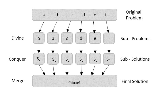
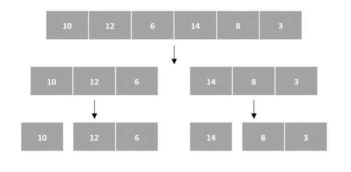
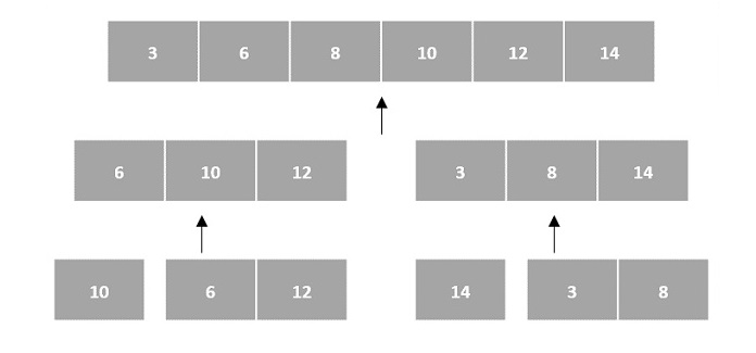
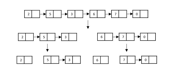
The Karatsuba method takes the divide and conquer approach by dividing the problem into multiple sub-problems and applies recursion to make the multiplication simpler.

Step 1

Assuming that n is the power of 2, rewrite the n-digit numbers in the form of −

X = 10n/2X1 + X2 Y = 10n/2Y1 + Y2

That gives us,

1456 = 102(14) + 56 
6533 = 102(65) + 33

First let us try simplifying the mathematical expression, we get,

(1400  6500) + (56  33) + (1400  33) + (6500  56) = 
104 (14  65) + 102 [(14  33) + (56  65)] + (33  56)

The above expression is the simplified version of the given multiplication problem, since multiplying two double-digit numbers can be easier to solve rather than multiplying two four-digit numbers.

However, that holds true for the human mind. But for the system compiler, the above expression still takes the same time complexity as the normal naive multiplication. Since it has 4 double-digit double-digit multiplications, the time complexity taken would be −

14  65 → O(4)
14  33 → O(4)
65  56 → O(4)
56  33 → O(4)
= O (16)

Thus, the calculation needs to be simplified further.

Step 2

X = 1456 
Y = 6533

Since n is not equal to 1, the algorithm jumps to step 3.

X = 10n/2X1 + X2 
Y = 10n/2Y1 + Y2

That gives us,

1456 = 102(14) + 56 
6533 = 102(65) + 33

Calculate Z = W (U + V) −

Z = (X1 + X2) (Y1 + Y2)  (X1Y1 + X2Y2) 
Z = X1Y2 + X2Y1 
Z = (14  33) + (65  56)

The final product,

P = 10n. U + 10n/2. Z + V 
   = 10n (X1Y1) + 10n/2 (X1Y2 + X2Y1) + X2Y2 
   = 104 (14  65) + 102 [(14  33) + (65  56)] + (56  33)

The sub-problems can be further divided into smaller problems; therefore, the algorithm is again called recursively.

Step 3

X₁ and Y₁ are passed as parameters X and Y.

So now, X = 14, Y = 65

X = 10n/2X1 + X2 
Y = 10n/2Y1 + Y2 
14 = 10(1) + 4 
65 = 10(6) + 5

Calculate Z = W (U + V) −

Z = (X1 + X2) (Y1 + Y2)  (X1Y1 + X2Y2) 
Z = X1Y2 + X2Y1 
Z = (1  5) + (6  4) = 29 

P = 10n (X1Y1) + 10n/2 (X1Y2 + X2Y1) + X2Y2 
   = 102 (1  6) + 101 (29) + (4  5) 
   = 910

Step 4

X₂ and Y₂ are passed as parameters X and Y.

So now, X = 56, Y = 33

X = 10n/2X1 + X2 
Y = 10n/2Y1 + Y2 
56 = 10(5) + 6 
33 = 10(3) + 3

Calculate Z = W (U + V) −

Z = (X1 + X2) (Y1 + Y2)  (X1Y1 + X2Y2) 
Z = X1Y2 + X2Y1 
Z = (5  3) + (6  3) = 33 

P = 10n (X1Y1) + 10n/2 (X1Y2 + X2Y1) + X2Y2 
= 102 (5  3) + 101 (33) + (6  3) 
= 1848

Step 5

X₁ + X₂ and Y₁ + Y₂ are passed as parameters X and Y.

So now, X = 70, Y = 98

X = 10n/2X1 + X2 
Y = 10n/2Y1 + Y2 
70 = 10(7) + 0 
98 = 10(9) + 8

Calculate Z = W (U + V) −

Z = (X1 + X2) (Y1 + Y2)  (X1Y1 + X2Y2) 
Z = X1Y2 + X2Y1 
Z = (7  8) + (0  9) = 56 

P = 10n (X1Y1) + 10n/2 (X1Y2 + X2Y1) + X2Y2 
= 102 (7  9) + 101 (56) + (0  8) 
=

Step 6

The final product,

P = 10n. U + 10n/2. Z + V

U = 910 
V = 1848 
Z = W  (U + V) = 6860  (1848 + 910) = 4102

Substituting the values in equation,

P = 10n. U + 10n/2. Z + V 
P = 104 (910) + 102 (4102) + 1848 
P = 91,00,000 + 4,10,200 + 1848 
P = 95,12,048

Analysis

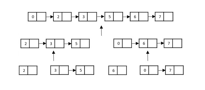
The Karatsuba algorithm is a recursive algorithm; since it calls smaller instances of itself during execution.

According to the algorithm, it calls itself only thrice on n/2-digit numbers in order to achieve the final product of two n-digit numbers.

Now, if T(n) represents the number of digit multiplications required while performing the multiplication,

T(n) = 3T(n/2)

This equation is a simple recurrence relation which can be solved as −

Apply T(n/2) = 3T(n/4) in the above equation, we get:
T(n) = 9T(n/4)
T(n) = 27T(n/8)
T(n) = 81T(n/16)
.
.
.
.
T(n) = 3i T(n/2i) is the general form of the recurrence relation 
of Karatsuba algorithm.

Recurrence relations can be solved using the masters theorem, since we have a dividing function in the form of −

T(n) = aT(n/b) + f(n), where, a = 3, b = 2 and f(n) = 0 
which leads to k = 0.

Since f(n) represents work done outside the recursion, which are addition and subtraction arithmetic operations in Karatsuba, these arithmetic operations do not contribute to time complexity.

Check the relation between a and b^k.

a > bk = 3 > 20

According to masters theorem, apply case 1.

T(n) = O(nlogb a)
T(n) = O(nlog 3)

The time complexity of Karatsuba algorithm for fast multiplication is O(n^{log 3}).

Example

In the complete implementation of Karatsuba Algorithm, we are trying to multiply two higher-valued numbers. Here, since the long data type accepts decimals upto 18 places, we take the inputs as long values. The Karatsuba function is called recursively until the final product is obtained.

CC++JavaPython

#include <stdio.h>#include <math.h>intget_size(long);longkaratsuba(long X,long Y){// Base Caseif(X <10&& Y <10)return X * Y;// determine the size of X and Yint size =fmax(get_size(X),get_size(Y));if(size <10)return X * Y;// rounding up the max length
   size =(size/2)+(size%2);long multiplier =pow(10, size);long b = X/multiplier;long a = X -(b * multiplier);long d = Y / multiplier;long c = Y -(d * size);long u =karatsuba(a, c);long z =karatsuba(a + b, c + d);long v =karatsuba(b, d);return u +((z - u - v)* multiplier)+(v *(long)(pow(10,2* size)));}intget_size(long value){int count =0;while(value >0){
      count++;
      value /=10;}return count;}intmain(){// two numberslong x =145623;long y =653324;printf("The final product is: %ld\n",karatsuba(x, y));return0;}

Output

The final product is: 95139000852

Strassen’s Matrix Multiplication is the divide and conquer approach to solve the matrix multiplication problems. The usual matrix multiplication method multiplies each row with each column to achieve the product matrix. The time complexity taken by this approach is O(n³), since it takes two loops to multiply. Strassens method was introduced to reduce the time complexity from O(n³) to O(n^{log 7}).

Naive Method

First, we will discuss Naive method and its complexity. Here, we are calculating Z=X Y. Using Naive method, two matrices (X and Y) can be multiplied if the order of these matrices are p q and q r and the resultant matrix will be of order p r. The following pseudocode describes the Naive multiplication −

Algorithm: Matrix-Multiplication (X, Y, Z) 
for i = 1 to p do 
   for j = 1 to r do 
      Z[i,j] := 0 
      for k = 1 to q do 
         Z[i,j] := Z[i,j] + X[i,k] × Y[k,j] 

Complexity

Here, we assume that integer operations take O(1) time. There are three for loops in this algorithm and one is nested in other. Hence, the algorithm takes O(n³) time to execute.

Strassens Matrix Multiplication Algorithm

In this context, using Strassens Matrix multiplication algorithm, the time consumption can be improved a little bit.

Strassens Matrix multiplication can be performed only on square matrices where n is a power of 2. Order of both of the matrices are n × n.

Divide X, Y and Z into four (n/2)×(n/2) matrices as represented below −

Z=[IKJL] X=[ACBD] and Y=[EGFH]

Using Strassens Algorithm compute the following −

M1:=(A+C)×(E+F)

M2:=(B+D)×(G+H)

M3:=(A−D)×(E+H)

M4:=A×(F−H)

M5:=(C+D)×(E)

M6:=(A+B)×(H)

M7:=D×(G−E)

Then,

I:=M2+M3−M6−M7

J:=M4+M6

K:=M5+M7

L:=M1−M3−M4−M5

Analysis

T(n)={c7xT(n2)+dxn2ifn=1otherwisewherecanddareconstants

Using this recurrence relation, we get T(n)=O(nlog7)

Hence, the complexity of Strassens matrix multiplication algorithm is O(nlog7).

Example

Let us look at the implementation of Strassen’s Matrix Multiplication in various programming languages: C, C++, Java, Python.

CC++JavaPython

#include<stdio.h>intmain(){int z[2][2];int i, j;int m1, m2, m3, m4 , m5, m6, m7;int x[2][2]={{12,34},{22,10}};int y[2][2]={{3,4},{2,1}};printf("The first matrix is: ");for(i =0; i <2; i++){printf("\n");for(j =0; j <2; j++)printf("%d\t", x[i][j]);}printf("\nThe second matrix is: ");for(i =0; i <2; i++){printf("\n");for(j =0; j <2; j++)printf("%d\t", y[i][j]);}
   m1=(x[0][0]+ x[1][1])*(y[0][0]+ y[1][1]);
   m2=(x[1][0]+ x[1][1])* y[0][0];
   m3= x[0][0]*(y[0][1]- y[1][1]);
   m4= x[1][1]*(y[1][0]- y[0][0]);
   m5=(x[0][0]+ x[0][1])* y[1][1];
   m6=(x[1][0]- x[0][0])*(y[0][0]+y[0][1]);
   m7=(x[0][1]- x[1][1])*(y[1][0]+y[1][1]);
   z[0][0]= m1 + m4- m5 + m7;
   z[0][1]= m3 + m5;
   z[1][0]= m2 + m4;
   z[1][1]= m1 - m2 + m3 + m6;printf("\nProduct achieved using Strassen's algorithm: ");for(i =0; i <2; i++){printf("\n");for(j =0; j <2; j++)printf("%d\t", z[i][j]);}return0;}

Output

The first matrix is: 
12	34	
22	10	
The second matrix is: 
3	4	
2	1	
Product achieved using Strassen's algorithm: 
104	82	
86	98

Let us consider a simple problem that can be solved by divide and conquer technique.

Max-Min Problem

The Max-Min Problem in algorithm analysis is finding the maximum and minimum value in an array.

Solution

To find the maximum and minimum numbers in a given array numbers[] of size n, the following algorithm can be used. First we are representing the naive method and then we will present divide and conquer approach.

Naive Method

Naive method is a basic method to solve any problem. In this method, the maximum and minimum number can be found separately. To find the maximum and minimum numbers, the following straightforward algorithm can be used.

Algorithm: Max-Min-Element (numbers[]) 
max := numbers[1] 
min := numbers[1] 

for i = 2 to n do 
   if numbers[i] > max then  
      max := numbers[i] 
   if numbers[i] < min then  
      min := numbers[i] 
return (max, min) 

Example

Following are the implementations of the above approach in various programming languages −

CC++JavaPython

#include <stdio.h>structPair{int max;int min;};// Function to find maximum and minimum using the naive algorithmstructPairmaxMinNaive(int arr[],int n){structPair result;
    result.max = arr[0];
    result.min = arr[0];// Loop through the array to find the maximum and minimum valuesfor(int i =1; i < n; i++){if(arr[i]> result.max){
            result.max = arr[i];// Update the maximum value if a larger element is found}if(arr[i]< result.min){
            result.min = arr[i];// Update the minimum value if a smaller element is found}}return result;// Return the pair of maximum and minimum values}intmain(){int arr[]={6,4,26,14,33,64,46};int n =sizeof(arr)/sizeof(arr[0]);structPair result =maxMinNaive(arr, n);printf("Maximum element is: %d\n", result.max);printf("Minimum element is: %d\n", result.min);return0;}

Output

Maximum element is: 64
Minimum element is: 4

Analysis

The number of comparison in Naive method is 2n – 2.

The number of comparisons can be reduced using the divide and conquer approach. Following is the technique.

Divide and Conquer Approach

In this approach, the array is divided into two halves. Then using recursive approach maximum and minimum numbers in each halves are found. Later, return the maximum of two maxima of each half and the minimum of two minima of each half.

In this given problem, the number of elements in an array is y−x+1, where y is greater than or equal to x.

Max−Min(x,y) will return the maximum and minimum values of an array numbers[x…y].

Algorithm: Max - Min(x, y) 
if y  x ≤ 1 then  
   return (max(numbers[x],numbers[y]),min((numbers[x],numbers[y])) 
else 
   (max1, min1):= maxmin(x, ⌊((x + y)/2)⌋) 
   (max2, min2):= maxmin(⌊((x + y)/2) + 1)⌋,y) 
return (max(max1, max2), min(min1, min2)) 

Example

Following are implementations of the above approach in various programming languages −

CC++JavaPython

#include <stdio.h>// Structure to store both maximum and minimum elementsstructPair{int max;int min;};structPairmaxMinDivideConquer(int arr[],int low,int high){structPair result;structPair left;structPair right;int mid;// If only one element in the arrayif(low == high){
        result.max = arr[low];
        result.min = arr[low];return result;}// If there are two elements in the arrayif(high == low +1){if(arr[low]< arr[high]){
            result.min = arr[low];
            result.max = arr[high];}else{
            result.min = arr[high];
            result.max = arr[low];}return result;}// If there are more than two elements in the array
    mid =(low + high)/2;
    left =maxMinDivideConquer(arr, low, mid);
    right =maxMinDivideConquer(arr, mid +1, high);// Compare and get the maximum of both parts
    result.max =(left.max > right.max)? left.max : right.max;// Compare and get the minimum of both parts
    result.min =(left.min < right.min)? left.min : right.min;return result;}intmain(){int arr[]={6,4,26,14,33,64,46};int n =sizeof(arr)/sizeof(arr[0]);structPair result =maxMinDivideConquer(arr,0, n -1);printf("Maximum element is: %d\n", result.max);printf("Minimum element is: %d\n", result.min);return0;}

Output

Maximum element is: 64
Minimum element is: 4

Analysis

Let T(n) be the number of comparisons made by Max−Min(x,y), where the number of elements n=y−x+1.

If T(n) represents the numbers, then the recurrence relation can be represented as

T(n)=⎧⎩⎨⎪⎪T(⌊n2⌋)+T(⌈n2⌉)+210forn>2forn=2forn=1

Let us assume that n is in the form of power of 2. Hence, n = 2^k where k is height of the recursion tree.

So,

T(n)=2.T(n2)+2=2.(2.T(n4)+2)+2…..=3n2−2

Compared to Nave method, in divide and conquer approach, the number of comparisons is less. However, using the asymptotic notation both of the approaches are represented by O(n).

Using divide and conquer approach, the problem in hand, is divided into smaller sub-problems and then each problem is solved independently. When we keep dividing the sub-problems into even smaller sub-problems, we may eventually reach a stage where no more division is possible. Those smallest possible sub-problems are solved using original solution because it takes lesser time to compute. The solution of all sub-problems is finally merged in order to obtain the solution of the original problem.

Broadly, we can understand divide-and-conquer approach in a three-step process.

Divide/Break

This step involves breaking the problem into smaller sub-problems. Sub-problems should represent a part of the original problem. This step generally takes a recursive approach to divide the problem until no sub-problem is further divisible. At this stage, sub-problems become atomic in size but still represent some part of the actual problem.

Conquer/Solve

This step receives a lot of smaller sub-problems to be solved. Generally, at this level, the problems are considered ‘solved’ on their own.

Merge/Combine

When the smaller sub-problems are solved, this stage recursively combines them until they formulate a solution of the original problem. This algorithmic approach works recursively and conquer & merge steps works so close that they appear as one.

Arrays as Input

There are various ways in which various algorithms can take input such that they can be solved using the divide and conquer technique. Arrays are one of them. In algorithms that require input to be in the form of a list, like various sorting algorithms, array data structures are most commonly used.

In the input for a sorting algorithm below, the array input is divided into subproblems until they cannot be divided further.

Then, the subproblems are sorted (the conquer step) and are merged to form the solution of the original array back (the combine step).

Since arrays are indexed and linear data structures, sorting algorithms most popularly use array data structures to receive input.

Linked Lists as Input

Another data structure that can be used to take input for divide and conquer algorithms is a linked list (for example, merge sort using linked lists). Like arrays, linked lists are also linear data structures that store data sequentially.

Consider the merge sort algorithm on linked list; following the very popular tortoise and hare algorithm, the list is divided until it cannot be divided further.

Then, the nodes in the list are sorted (conquered). These nodes are then combined (or merged) in recursively until the final solution is achieved.

Various searching algorithms can also be performed on the linked list data structures with a slightly different technique as linked lists are not indexed linear data structures. They must be handled using the pointers available in the nodes of the list.

Pros and cons of Divide and Conquer Approach

Divide and conquer approach supports parallelism as sub-problems are independent. Hence, an algorithm, which is designed using this technique, can run on the multiprocessor system or in different machines simultaneously.

In this approach, most of the algorithms are designed using recursion, hence memory management is very high. For recursive function stack is used, where function state needs to be stored.

Examples of Divide and Conquer Approach

The following computer algorithms are based on divide-and-conquer programming approach −

• Max-Min Problem
• Merge Sort Algorithm
• Quick Sort Algorithm
• Binary Search Algorithm
• Strassen’s Matrix Multiplication
• Karatsuba Algorithm
• Closest pair (points)

There are various ways available to solve any computer problem, but the mentioned are a good example of divide and conquer approach.