Category: AI – Constraint Satisfaction

Solving Traveling Sales Problem with CSP Algorithms

The Traveling Salesperson Problem (TSP) is to find the shortest path that travels through each city exactly once and returns to the starting city. As a Constraint Satisfaction Problem the variables, domains, and constraints of Traveling Sales Problem are listed below −

• Variables: The Cities (nodes) are variables in the graph.
• Domain: Any city that a salesperson visits except those cities already visited.
• Constraints: Each city is visited exactly once. The traveler returns back to the start city with minimized total travel distance.

Backtracking

Backtracking is a deep-search method which is used to find a solution for complex problems. First we assign a value to the variable from its domain by following the constraint step by step and if we find the constraint is violated we go back and try a different value for previous variables.

This code utilizes backtracking to find valid paths and decide which solution is best given the following constraints.

Step 1: Define the Problem

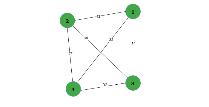
The graph is represented as a distance matrix. Here, graph[i][j] indicates the distance between City i and City j. For example, if graph[0][1] = 12, then the distance between City 1 and City 2 is 12 units.

Here, n refers to the total number of cities, and start_node refers to the city through which the algorithm begins searching for possible routes. This structure can be seen as a basic path-finding for solving Constraint Satisfaction Problem (CSP) approaches.

# The first step is to define the graph with nodes and edges representing cities and their distances.# Graph represented as a distance matrix
graph =[[0,12,17,22],# Distances from node 1[12,0,27,38],# Distances from node 2[17,27,0,32],# Distances from node 3[22,38,32,0]# Distances from node 4]
n =len(graph)# Number of nodes
start_node =0# Starting from node 1 (index 0)

Step 2: Define the TSP Solver Class

The TSP solver uses backtracking to explore all possible paths and find the optimal solution.

The graph and start_node are stored, and variables are initialized to track the best path and minimum cost (best_path and min_cost).

classTSP:def__init__(self, graph, start_node):
      self.graph = graph
      self.start_node = start_node
      self.best_path =None
      self.min_cost =float('inf')defsolve(self):
      visited =[False]*len(self.graph)
      visited[self.start_node]=True
      self.backtrack([self.start_node],0, visited)return self.best_path, self.min_cost
   
   defbacktrack(self, path, current_cost, visited):# Base case: All nodes visited, return to the startiflen(path)==len(self.graph):
         total_cost = current_cost + self.graph[path[-1]][self.start_node]if total_cost < self.min_cost:
            self.min_cost = total_cost
            self.best_path = path +[self.start_node]return# Try all possible next nodesfor next_node inrange(len(self.graph)):ifnot visited[next_node]and self.graph[path[-1]][next_node]>0:
            visited[next_node]=True
            self.backtrack(path +[next_node], current_cost + self.graph[path[-1]][next_node], visited)
            visited[next_node]=False

Step 3: Solve the TSP Problem

We create an instance of the TSP class and call the solve method.

The solver (solve method) is then invoked to compute the optimal path and minimum cost, starting from the specified node and traversing the graph using backtracking logic.

tsp = TSP(graph, start_node)
best_path, min_cost = tsp.solve()# Output the resultsprint("Optimal Path:",[node +1for node in best_path])# Convert to 1-based indexingprint("Minimum Cost:", min_cost)

Complete Code

The Traveling Sales Problem (TSP) solver’s complete implementation is shown below, which uses backtracking to determine the optimal path with the lowest cost.

# Graph represented as a distance matrix
graph =[[0,12,17,22],[12,0,27,38],[17,27,0,32],[22,38,32,0]]
n =len(graph)  
start_node =0classTSP:def__init__(self, graph, start_node):
      self.graph = graph
      self.start_node = start_node
      self.best_path =None
      self.min_cost =float('inf')defsolve(self):
      visited =[False]*len(self.graph)
      visited[self.start_node]=True
      self.backtrack([self.start_node],0, visited)return self.best_path, self.min_cost
   
   defbacktrack(self, path, current_cost, visited):iflen(path)==len(self.graph):
         total_cost = current_cost + self.graph[path[-1]][self.start_node]if total_cost < self.min_cost:
             self.min_cost = total_cost
             self.best_path = path +[self.start_node]returnfor next_node inrange(len(self.graph)):ifnot visited[next_node]and self.graph[path[-1]][next_node]>0:
            visited[next_node]=True
            self.backtrack(path +[next_node], current_cost + self.graph[path[-1]][next_node], visited)
            visited[next_node]=False
         
tsp = TSP(graph, start_node)
best_path, min_cost = tsp.solve()# Output the resultsprint("Optimal Path:",[node +1for node in best_path])print("Minimum Cost:", min_cost)

Following is the output of the above code −

Optimal Path: [1, 2, 3, 4, 1]
Minimum Cost: 93

Constraint Satisfaction problems (CSP) is a mathematical problem defined by a set of variables, their possible values (domain), and constraints that limit the ways in which the values can be combined.

CSPs has methods to systematically investigate possible solutions while avoiding dead end paths in order to solve efficiently. Following are various methods to solve CSPs −

• Backtracking Algorithm
• Forward-Checking Algorithm
• Constraint Propagation Algorithms
• Local Search

Backtracking Algorithm

Backtracking is a deep-first search method, which is a recursive algorithm for solving problems that require searching for solutions in a structured space. It checks all possible sequences of decisions, stopping when it detects a solution or determines that no solution exists.

The approach tries to construct a solution slowly, adding one variable at a time. When it determines that the current solution cannot be stretched into a valid solution, it “backtracks” the previous decision by trying with a different value.

We can improve backtracking by choosing the variable with the most constraints. The idea is to deal with the most “tough” or “sensitive” variables first. The backtracking algorithm has the following components −

• Variable Ordering: Choosing which variable to assign a value to next in the search process is called variable ordering. Picking the right order can make the algorithm work much better.For instance, in Sudoku, if we start solving variables with the smallest number of available choices (almost negligible variables), we will decrease the number of decisions that we need to do for the rest of the variables. The idea is called Minimum Remaining Values or MRV which means we need to solve first variables with the least number of valid options.
• Value Ordering: Once we have determined which variable to assign (Variable Ordering), we must choose which value from its domain to test first. The order in which we assign values also influences the performance of the algorithm.For instance, in a map coloring problem, assigning a color which causes the least conflict between neighbor regions is a smoother search, and this is known as Least Constraining Value (LCV) heuristic, where we try values that leave the most flexibility for other variables.

Working of Backtracking Algorithm

Following are the steps for Backtracking Algorithm −

• Step 1: Assign a value to the variable based on the problems constraints.
• Step 2: After assigning a value, check if the current assignment is valid based on the constraints.
• Step 3: Move to the next variable and repeat the process.
• Step 4: If assigning a value violates a constraint or leads to no valid solutions, undo the assignment (backtrack) and try with different value.
• Step 5: Continue until a solution is found or all possibilities have been exhausted.

Advantages

This approach has the following advantages −

• It is easy to implement for many problems.
• Works for a wide variety of problems by changing the constraints.
• It guarantees finding a solution if one exists.

Limitations

Despite its strengths, backtracking has certain drawbacks −

• For large problems, it may take too long as it explores many possible paths.
• It may repeatedly explore the same invalid paths without optimization.

Forward-Checking Algorithm

In order to solve a CSP, we use search algorithms that assign values to variables one at a time; however, limitations may make certain assignments incorrect. Forward-Checking (FC) is a technique used during this search process to avoid wasting time on invalid assignments.

Forward checking is an algorithmic reduction technique that minimizes the domains of unassigned variables immediately after assigning a value to a variable. This is achieved by comparing constraints between assigned and unassigned variables. The constraint violates if any value in the domain of an unassigned variable matches with the allocated variables then that value will be removed.

Working of Forward-Checking Algorithm

Following are the steps for Forward checking algorithm −

• Choose a variable, and assign to it a value.
• Look at the constraints between the assigned variable and all other unassigned variables.
• Remove values from the domains of unassigned variables if they violate the constraint.
• If any unassigned variables domain becomes null, backtrack immediately (because no solution is possible with the current assignment).

Advantages

The forward-checking method has following advantages −

• Reduces the size of the search space by removing inconsistent values first.
• Detects dead ends earlier than the backtracking algorithm.
• Increases efficiency in numerous CSPs.

Limitations

However, forward-checking has certain limitations that can affect its effectiveness −

• Forward-checking only examines one step ahead, therefore it may still investigate improper paths where constraints between unassigned variables are violated. When combined with techniques such as constraint propagation (e.g., arc consistency), all constraints are maintained consistently.

Constraint Propagation Algorithms

Constraint propagation is a strategy that solves CSPs by reducing variable’s possible values or domains by successively applying a set of constraints.

Unlike forward-checking, which checks one step forward, constraint propagation ensures that all possible constraints between any connected variables are consistent by modifying the domains of all pairs rather than just immediate ones.

This technique gradually eliminates the choices of each variable, which makes the problem easier to solve by eliminating wrong choices early. It encourages consistency throughout the task and prevents the algorithm from following wrong paths, saving time and computing effort.

The common methods that are used in constraint propagation are described below −

Arc Consistency

This method ensures that any value of one variable corresponds to a valid value in another related variable −

• Step 1: Start with a CSP problem, including the variables, their domains, and constraints between variables.
• Step 2: Iterate over all arcs of constraints among variables. Verify that every value in the domain of one variable maps to a consistent value in the domain of the other variable.
• Step 3: When an inconsistency is found, delete the incorrect values from the first variable’s domain and check the affected arcs.
• Step 4: Repeat this process until all arcs are consistent or a domain becomes empty, which indicates the need to backtrack and revise previous assignments.

Node consistency

This method make sure that individual variables meet the constraints applied to them. When a value in a variable’s domain violates a constraint, it is removed. For example, if a meeting room is not large enough for a team, remove it from the list of options.

Path consistency

This method checks triples of variables and ensures that the relations among them are consistent. For example, if X = 1 and X + Y = Z, then path consistency ensures the domain for Z has valid numbers based on X and Y.

Advantages

Constraint propagation has these benefits −

• This method reduces variable domains, making it easier to identify a solution.
• Detects inconsistencies early as compared to other algorithms, hence saving time and money.

Limitations

This method has following disadvantages −

• If the problem is large, complex and has many variables and constraints this method will be slow.
• May not fully solve the problem and often needs to be go back to complete the process.

Local Search

Local Search is a problem-solving method that involves researching the “neighborhood” of possible solutions. It does not search the entire solution space but starts with an initial solution and improves it gradually by making minor changes.

The objective is to find a good enough solution rather than exhaustively searching for the perfect one, which makes it suitable for huge and complex problems. Let us understand Local Search by using an example −

• This example is about class scheduling, let us begin with an random schedule which assigns classes to the time slots and rooms, even in case of conflicts.
• Class A: Room 1, 9:00 AM, class B: Room 1, 9:00 AM (Conflict: same room and time) and class C: Room 2, 10:00 AM
• Minimize conflicts in scheduling for example no two classes should have the same room at the same time.
• Reschedule by shifting one class to a different room or time slot. For instance: Shift Class B to Room 2 at 9:00 AM.
• Find the conflicts in the current schedule. In our case conflicting is class B. Shift it to a new room or time that reduces conflicts.
• We can end this when all conflicts have been resolved, such that no classes overlap, or a time limit is reached.

Advantages

Local search methods has the following benefits for solving CSPs −

• Works well for large, complex problems.
• Quickly finds “good enough” solutions.
• Easy to implement and understand.

Limitations

Despite its advantages, local search has a few drawbacks −

• In local search, the algorithm might find a solution that seems good, but it’s not the best possible. It might stop searching once it finds a “good enough” solution, missing the best one.
• Local search methods need to be adjusted for each problem, as what works for one may not work for another.

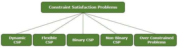
Constraint Satisfaction Problems (CSPs) are categorized based on their structure and the complexity of the constraints they involve. These problems vary from simple binary constraints to more complex, dynamic, and over-constrained problems. The categories help determine which method is most suitable for solving these problems efficiently. Some common categories include −

Dynamic CSPs (DCSPs)

Dynamic Constraint Satisfaction Problems (DCSPs) is a variation of traditional CSPs, where variables and constraints change over time. The problems are flexible and thus require algorithms that can change as the problem evolves. The problem evolves due to external variables or environmental adjustments.

• Adding or removing constraints and variables in DCSPs increases the complexity of problems.
• For example, In real-time scheduling, the variable could be the availability of resources or timing of the task in which they might change in the process of solving the problem.
• The problem with DCSPs is that the solutions obtained should always be evaluated and changed as constraints evolve.
• The solving strategies depend on previously found solutions to help the newly introduced problem solution and manage changes effectively.

Solving Dynamic CSPs

DCSP problem-solving methodologies prioritize the use of solution information from previous solutions to efficiently solve complicated situations as they arise. These strategies can be categorized based on how information is conveyed between consecutive problem situations. The solving methods are as follows −

Oracles

Oracle is a method for solving new problems by applying solutions from prior ones. Instead of beginning from scratch, they reuse previous solutions to save time and effort.

For example, let us assume you are managing a meal delivery schedule. Yesterday, you determined the best route for your drivers. Today’s orders are slightly different, but most of the previous routes are still applicable. Instead of starting from scratch, you use yesterday’s schedule to help you navigate today’s orders.

Local repair

Local repair is like repairing a partially broken toy. Instead of discarding it, you alter it a little to make it work again. Here, you are applying the solution from the previous CSP to “repair” the parts that no longer fit because of the new changes.

For instance, let us assume the seating chart for 50 guests. Two guests canceled and three more confirmed. Instead of making a new chart, you adjust the chart with the changes. Thus, you save much time without losing functionality.

Constraint Recording

Constraint recording is similar to learning from failure. Each time you solve an issue, you start seeing trends and remember the rules that worked or did not work. These lessons are applied to the next task so that time and errors are saved, and not repeated.

For example, consider planning a weekly basketball tournament. First week, you find out teams take at least 30 minutes between games to warm up. So you add it as a rule (constraint) and apply this to all schedules. Every week you learn something and use that knowledge to improve the program.

Example use case of Dynamic CSP

A classic example of a Dynamic CSP is a problem of real-time scheduling in which −

• Resources like workers and machines become available and unavailable over time.
• Task durations and deadlines may change if new tasks are added or current ones are rescheduled.
• Task constraints vary depending on changes in the environment such as precedence and resource constraints.

In such cases, solving approaches such as local repair or constraint recording enable the algorithm to adapt and deliver solutions that account for the problem’s dynamic character.

Flexible CSPs

Flexible CSPs are a type of problem where not all the rules have to be strictly followed. In traditional CSPs, all conditions need to be satisfied, but flexible CSPs have some rules to be adjusted or even partially ignored so that answers can be found easily in real situations where it may not be possible to follow all the rules.

• For example, in AI-based exam scheduling, a flexible CSP may permit overlapping tests for a small set of students if it results in a better schedule for the rest.

Solving flexible CSPs

Flexible CSPs focuses on following as many rules as possible or giving priority to the most important ones. The solving methods are as follows −

MAX-CSP

In this approach, some constraints may need to be violated with the goal of maximizing the number of constraints satisfied.

For instance, in conference scheduling problems, some sessions will overlap each other since there exists a limited number of rooms. The algorithm aims at scheduling as many sessions as possible without conflicts by tolerating some overlaps.

Weighted CSP

This is an extension of MAX-CSP where weight or priority is assigned to each constraint. Higher-weighted constraints are prioritized and addressed first in the solution.

For example, in an AI-powered robot navigation system, avoiding obstacles in the way (high weight)-is prioritized over the quicker route (low weight). By providing these rules, the robot focuses on high-weight of safety while navigating even if it means traveling a little longer distance.

Fuzzy CSP

In fuzzy CSPs, constraints are considered as flexible relations, with satisfaction measured on a scale of fully satisfied to fully violated. The goal is to create a solution that maximizes satisfaction while meeting all restrictions.

For example, the ideal room temperature can be set by a smart thermostat system to be between 22C and 24C. Temperatures that are somewhat higher or lower, for example, 21C or 25C, could also be acceptable. The system would try to keep the temperature as close as possible to the optimal range.

Binary CSPs

A Binary Constraint Satisfaction Problem (Binary CSP) has variables and constraints with every constraint defined between two variables. This type of CSP is critical for constraint resolution because every generic CSP can be translated to an equivalent binary CSP. In a Binary CSP −

• Variables have specific domains (possible values).
• Constraints specify the permissible value combinations for pairs of variables.

Binary CSPs are usually used in modeling the interactions of pairs of elements in situations such as graph coloring, scheduling, and resource allocation.

Solving Binary CSPs

Several methods can be used to solve binary CSPs, including −

Backtracking

Backtracking is a trial and error where we assign values to variables step by step and check whether they satisfy the constraints. First, we assign a value to the first variable from its domain and move to the next variable. If we find that a constraint is violated, we go back and try a different value for the previous variable.

Constraint Propagation

This method is like just cleaning up before beginning. It makes the search easier by getting rid of choices that won’t work right from the start.

• Arc Consistency: The AC-3 algorithm gets rid of all pairs where a value from one variable’s options doesn’t match up with a value from another variable’s options. Let’s say x1 can be {1,2} and x2 can be {2,3}, and they need to follow the rule x1<x2. AC-3 will take 2 out of x1’s options because having 2 for x1 doesn’t allow x1<x2 to be true.

Forward Checking

This method avoids getting stuck in dead ends. After assigning a value to a variable, it checks the domains of the remaining unassigned variables and eliminates the values that no longer apply. If any of the domains becomes empty, backtrack and try another value. It is a good approach because it stops us earlier if there isn’t a solution and saves more time than just continuing blindly.

Graph-Based Approaches

Binary CSPs can be graphically represented by considering the following −

• Nodes = Variables.
• Edges = constraints.

Graph-based approaches make the problem simpler:

• Tree Decomposition: The graph is broken down into smaller tree-like structures, and then each one of them is solved separately and their results are combined.
• CutSet Conditioning: The graph is reduced by eliminating a small set of variables; solve the simplified problem and then correct the result for the original problem.

Non-binary CSPs

Non-binary CSPs are constraint satisfaction problems with three or more variables, whereas binary CSPs have only two variables. These problems are common in real-world scenarios where many variables’ relationships need to be considered at the same time. Examples of non-Binary CSPs −

• Sudoku puzzles, which require unique numbers in each 3×3 sub-grid and have constraints on 9 variables.
• Class Scheduling: Assigning teachers, time slots, and classrooms to courses limits many variables.

Non-binary CSPs are hard since the complexity increases with the number of variables involved in the constraints. Much harder to represent and solve directly than binary CSPs.

Solving non-binary CSPs

To solve non-binary CSPs, a variety of methods can be used, often by transforming them into binary CSPs or by using special techniques −

Direct solving

In this approach, we try to solve the problem directly by working with the original constraints that contain many variables rather than simplifying or reducing them first. This solution does not require extra effort to change the problem, so it is faster in some situations. It can be slow if the problem is complex because we are dealing with a lot of data.

Reduction to binary CSPs

This method divides a huge, complex problem into smaller ones using only two variables at a time. If you have a constraint like X + Y + Z = 10, instead of solving for all three variables at once, define a new variable W as X + Y. Now, the problem is W + Z = 10, which is easier to solve because it only has two variables (W and Z) rather than three.

Over Constrained Problems

Over-constrained means that there are too many, or even extreme, limitations placed upon the problem; hence, developing a solution is difficult as the solution has to satisfy all these at once.

In CSP words, it occurs when the number of constraints exceeds the number of potential solutions, or when the constraints are too incompatible to be met simultaneously. Examples of over constrained problems are −

• Map Coloring: Let us assume that we had a map with ten regions and six colors, but each region on the map could not be coloured with the same color as any one of its neighboring regions, it might become impractically constraining if these restrictions (relation of adjacency) are too restrictive to be met by the available colors.
• Job Scheduling: In this example, we need to plan ten tasks in three-time slots, where the constraint is certain tasks do not overlap in time and some tasks should be finished first. So with only three slots, we cannot find a valid schedule.

Solving Over-Constrained Problems

To handle over-constrained problems we can use two methods −

A Constraint Satisfaction Problem (CSP) is used to find a solution that involves following a predefined conditions and rules. It is commonly used in puzzle solving, or in resource scheduling where resources allocated based on certain constraints and task planning where constraint include following a specific order.

Three primary components that make up the representation of Constraint Satisfaction Problems (CSP): variables, domains, and constraints.

• Finite Set of Variables (V1,V2,…,Vn): The unknowns in the problem that require values are represented by variables. For instance, classroom seating arrangement problem, the variables are V1, V2, and V3, which stands for a student who needs to be seated.
• Non-Empty Domains (D1,D2,…,Dn): Every variable has a domain of potential values. For instance, seating arrangement problem. D1={Seat1, Seat2, Seat3} V1(Student 1), D2={Seat1, Seat2, Seat3} V2 (Student 2), and so on. Each student’s possible seat availability is specified by the domain.
• Finite Set of Constraints (C1,C2,…,Cn): Constraints limit the values that variables can take by defining their relationships.

In a CSP, we deal with many types of restrictions on variables. Constraints help narrow down our choices to get an appropriate solution of the problem. Depending upon the number of variables affected, constraints can either be unary, binary, or of some higher order.

• Unary Constraints: Apply to a single variable. For example: V1Seat1 (Student 1 cannot sit in Seat 1).
• Binary Constraints: Involve two variables. For example: V1V2 (No two students can occupy the same seat).
• Higher-Order Constraints: Involve three or more variables. For instance: V1,V2,V3 must all have distinct seat assignments.

Below is a detailed representation, along with examples and additional concepts like graph representation and arc-consistency.

Representation of Constraints in CSPs

This section covers the representation and management of CSPs. A constraint graph is a visualization tool where nodes are used to represent variables, and edges show constraints between variables. Mathematical expressions supplement this by defining the scope of restrictions (the set of variables involved) as well as valid value combinations for those variables.

All of these representations come together to form a very solid basis from which one can understand and effectively solve CSPs. Below, we explore graphical representation, mathematical formulation, and the concept of arc-consistency in detail.

Graphical Representation of CSP

A constraint graph is a graphical tool used to represent Constraint Satisfaction Problems (CSPs). It serves as a visualization of the variables’ interactions with their constraints. It simplifies the structure of the problem to allow for easier analysis and solving.

• Nodes: Represent the CSP’s variables.
• Edges: Edge indicates connection between two variables. If there is a constraint between two variables, an edge connects the nodes.

Example

In the classroom seating problem, the variables V1, V2, and V3 each represent a student’s seat, and the constraint is no two students sit in the same seat.

• Nodes: V1: seat for student 1, V2: seat for student 2, V3: seat for student 3
• Edges: V1 V2, V2 # V3, V1 V3 no students can be seated in the same seat.

The nodes represent the variables (seats for the students), edges represent constraints between the variables.

Advantages of using Graphical Representation

Following are the advantages of using graphical representation in CSP −

• Constraint graphs offer a clear and understandable representation of problems.
• Constraint graphs are useful for both large and small problems.
• It provides a clear and intuitive way to visualize the relationships between variables and constraints.
• Constraint graphs are applied in the backtracking algorithm and constraint propagation to solve CSPs in an efficient way.

Mathematical Representation of Constraints

In a mathematical representation of constraints in a CSP, each constraint is defined by a scope and a relation. The following is a mathematical representation of constraints: <Relation, Scope>. These relations represent the possible pairs of values that satisfy the specified constraint.

• Scope: The set of variables that involved in the constraint.
• Relation: A list of possible values that the variables can have.

Example

The following example illustrates how to represent constraints mathematically in a CSP. It illustrates the relationship between variables and their valid value combinations by using a specific situation where two variables cannot have the same value.

• Constraint: V1V2
• Scope: {V1,V2} (constraint-related variables).
• Relation: {(Seat1, Seat2),(Seat2, Seat3),(Seat1, Seat3)} are valid combinations of values for V1 and V2.

Advantages of Mathematical Representation

Following are the advantages of mathematical representation and when to use it −

• This is useful whenever you want to state and define constraints in an accurate and systematic way.
• Useful for theoretical CSP analysis that requires demonstrating relationships between variables and their domains.

Arc-Consistency

Arc-consistency simplifies CSPs by reducing the domain of variables. A variable is arc-consistent if every value in its domain satisfies all constraints with the connected variables. This method is repeated recursively for all variables and constraints until no further domain reductions are possible, thus ensuring that the CSP is fully arc-consistent.

Example

This example illustrates how arc-consistency works on CSPs, by the decreasing the scope of variables gradually. It ensures that no value in one variable’s domain clashes with the constraints involving by related variables, thus making the problem-solving process easier.

• Constraint: V1 V2.
• Domain of V1: {Seat1, Seat2, Seat3}.
• Domain of V2: {Seat1, Seat2, Seat3}.

If V1=Seat1, seat1 must be removed from V2’s domain to avoid violating the condition V1V2. This method continues until all variables are arc-consistent, which reduces the search space.

Advantages of Arc-Consistency

• Arc-consistency enforcement improves problem-solving efficiency because it reduces incorrect possibilities as early as possible, thus reducing the overall search space and limits the need of backtracking.
• This method helps to speed up the solution process by ensuring consistency between variables and reducing the complexity of the problem.

Note: Arc-consistency reduces the complexity of the problem but it doesn’t guarantee an exact solution to all CSP problems additional algorithms are necessary for harder tasks.

Constraint Satisfaction Problem (CSP) has a big impact on artificial intelligence (AI) when solving problems that need solutions to follow certain rules or limits. CSP helps to fix real-world issues that involve making choices based on limits, like setting up schedules, dividing up resources, making plans, and solving sudoku puzzles.

CSPs solve complex problems by breaking them into structured parts by identifying constraints that must be satisfied to find a solution. By using algorithms made to satisfy constraints, AI can handle tasks from puzzle-solving to optimizing workflows, better in fields like shipping, robotics, and manufacturing.

What is the Constraint Satisfaction Problem?

A Constraint Satisfaction Problem (CSP), is a mathematical problem that aims to find values for variables by satisfying constraints or criteria. In the problem, each variable is assigned a domain, which represents the set of values it is allowed to accept. Constraints represent the relationships among variables, restricting the values they can simultaneously take.

• For example, the N-Queens problem considers a variable such as the placement of queens on the board, values are considered as rows or columns where a queen can be put, and the constraints are no two queens must share the same row, column, or diagonal.
• Techniques for solving a CSP include backtracking, forward checking, and constraint propagation, which search for feasible values and solutions efficiently.

Components of Constraint Satisfaction Problem

In a Constraint Satisfaction Problem (CSP), a solution is represented as a tuple of variables with values that satisfy all constraints. Here are the key components for creating and solving a CSP −

Variables

Variables in CSP represent the elements or entities that require value determination. They refer to the problem’s unknown values that need to determined to obtain a solution.

For example, in a map coloring problem, one of the possible variables includes regions that need to be assigned colors.

Domains

Domains are sets of possible values that a variable can take. These can be infinite or finite depending on the problem. For example, in scheduling problems, the domain can be a time slot that is likely the hours between 9 AM and 5 PM assigned to any tasks.

There are four kinds of domains based on their nature: finite, infinite, discrete, and continuous domains each defines what values a variable can take for a given problem.

• Finite Domains: A domain that has a narrow range of possible values. In this domain we will have fixed list of values and we cannot pick anything outside of that domain.For example, the domain for the time slots in a daily scheduling problem could be {9:00 am, 10:00 am, 11:00 am, 12:00 am} and we cannot pick 9:30 am or 10:30 am because they are not in the variable’s domain.
• Infinite Domains: A domain that can take any value and all real numbers. We are not limited to fixed set of values we can take infinite number of values i.e, outside of the domain.For example, for a fluid flow problem, the pressure of the liquid can be any real number from 0 to 1000 Pascals or when measuring a height of the tree, height can be 5.01m, 5m or 5.0001m no matter how precisely we calculate, we will always have lot of possible values.
• Discrete Domains: A domain that has distinct, separated values, and countable with no immediate values between them.For example, the quantity of people in a hall is represented by the notation {0, 1, 2,…} but it cannot be 1.5, 2.5, 3.001.. because a person cannot be split into half it should be whole and distinct meaning it should be continuous and no in between values
• Continuous Domains: A domain that covers all the possible values in a given range with unlimited precision. These are very much used in measurements and real world physics.For example, in a room the temperature can range between 15C and 30C.

Constraints

Constraints are rules that limit the ways in which variables can interact with one another. They ensure that the assigned values meet the problem’s requirements.

For example, a constraint in a Sudoku puzzle might be that each number from 1 to 9 can only appear once in each row, column, and 3×3 grid.

Applications of Constraint Satisfaction Problem

CSPs are frequently used in real-world applications to model and solve decision-making problems with specific constraints. Some significant applications are given below −

• Scheduling: Allocation of resources such as people, tools, or rooms among projects, by ensuring that time and availability constraints are satisfied. For example, scheduling employees meetings or shifts to avoid issues.
• Planning: Planning is organization of activities or tasks in a specific sequence so that each will be completed within the required time and in the correct sequence. This is like a following a recipe or building a house where next tasks depends on the previous one. This is most commonly applied in robotics and project management when decisions are made based on the result of prior tasks.
• Resource allocation: Distribution of resources (such as funds, labor, or equipment) to prevent overuse and guarantee the best results. For instance, distributing funds among departments while respecting financial constraints.
• Puzzle Solving: Solving puzzle problems in which variables such as numbers or positions must be assigned in a method that obeys certain constraints: Sudoku, or the N-Queens problem. The process of finding a correct answer, where each assignment has to comply with the rules.

Benefits of Constraint Satisfaction Problems

CSP has several benefits that make it an effective tool for solving complex problems. Here are some key advantages −

• CSPs help decision-makers by finding solutions that best meet all relevant constraints.
• CSPs are effective for both small and large problems, making them flexible to various settings.
• Many CSP algorithms can solve problems automatically. This saves time and reduces errors.
• CSPs manage two sorts of constraints: hard constraints and soft constraints. Hard constraints must be strictly followed, but soft constraints are preferences or guidelines that can be altered based on priority. This makes them highly flexible to a variety of problems.

Challenges in Solving Constraint Satisfaction Problems

Solving Constraint Satisfaction Problems (CSPs) can be difficult because of various aspects. The following are some key difficulties −

• As the number of variables and constraints increases, solving CSPs becomes computationally expensive and time-consuming.
• Constraint conflicts occur when a problem’s conditions collide, making a solution impossible. For example, if two classes require separate rooms at the same time but only one room is available, the issue cannot be solved.
• If the constraints change often, solving the CSP again could be expensive. For instance, rescheduling flights multiple times due to unexpected changes in weather conditions requires recalculating routes and crew assignments.
• Most often solving very large CSPs with hundreds of variables or constraints is difficult and requires a lot of computation.