Category: Approximation Algorithms

  • Travelling Salesman using Approximation Algorithm

    We have already discussed the travelling salesperson problem using the greedy and dynamic programming approaches, and it is established that solving the travelling salesperson problems for the perfect optimal solutions is not possible in polynomial time.

    Therefore, the approximation solution is expected to find a near optimal solution for this NP-Hard problem. However, an approximate algorithm is devised only if the cost function (which is defined as the distance between two plotted points) in the problem satisfies triangle inequality.

    The triangle inequality is satisfied only if the cost function c, for all the vertices of a triangle u, v and w, satisfies the following equation

                     c(u, w) c(u, v)+c(v, w)
    

    It is usually automatically satisfied in many applications.

    Travelling Salesperson Approximation Algorithm

    The travelling salesperson approximation algorithm requires some prerequisite algorithms to be performed so we can achieve a near optimal solution. Let us look at those prerequisite algorithms briefly −

    Minimum Spanning Tree − The minimum spanning tree is a tree data structure that contains all the vertices of main graph with minimum number of edges connecting them. We apply prims algorithm for minimum spanning tree in this case.

    Pre-order Traversal − The pre-order traversal is done on tree data structures where a pointer is walked through all the nodes of the tree in a [root left child right child] order.

    Algorithm

    Step 1 − Choose any vertex of the given graph randomly as the starting and ending point.

    Step 2 − Construct a minimum spanning tree of the graph with the vertex chosen as the root using prims algorithm.

    Step 3 − Once the spanning tree is constructed, pre-order traversal is performed on the minimum spanning tree obtained in the previous step.

    Step 4 − The pre-order solution obtained is the Hamiltonian path of the travelling salesperson.

    Pseudocode

    APPROX_TSP(G, c)
       r <- root node of the minimum spanning tree
       T <- MST_Prim(G, c, r)
       visited = {}
       for i in range V:
          H <- Preorder_Traversal(G)
          visited = {H}
    

    Analysis

    The approximation algorithm of the travelling salesperson problem is a 2-approximation algorithm if the triangle inequality is satisfied.

    To prove this, we need to show that the approximate cost of the problem is double the optimal cost. Few observations that support this claim would be as follows −

    • The cost of minimum spanning tree is never less than the cost of the optimal Hamiltonian path. That is, c(M) c(H*).
    • The cost of full walk is also twice as the cost of minimum spanning tree. A full walk is defined as the path traced while traversing the minimum spanning tree preorderly. Full walk traverses every edge present in the graph exactly twice. Thereore, c(W) = 2c(T)
    • Since the preorder walk path is less than the full walk path, the output of the algorithm is always lower than the cost of the full walk.

    Example

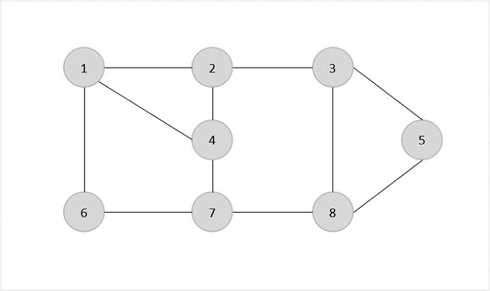
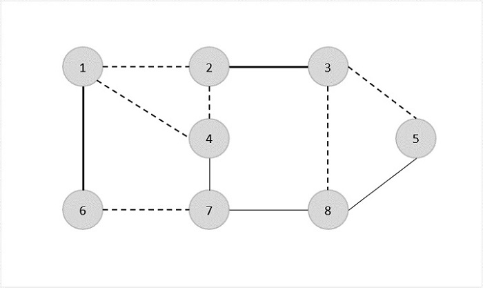
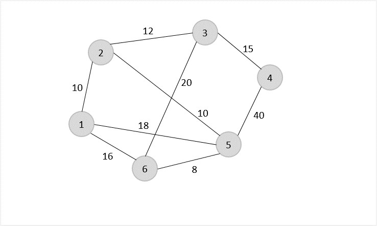
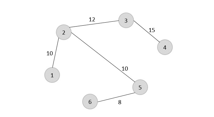
    Let us look at an example graph to visualize this approximation algorithm −

    approximation_algorithm

    Solution

    Consider vertex 1 from the above graph as the starting and ending point of the travelling salesperson and begin the algorithm from here.

    Step 1

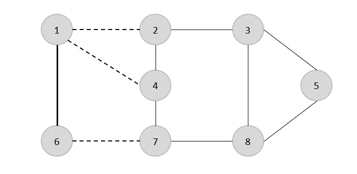
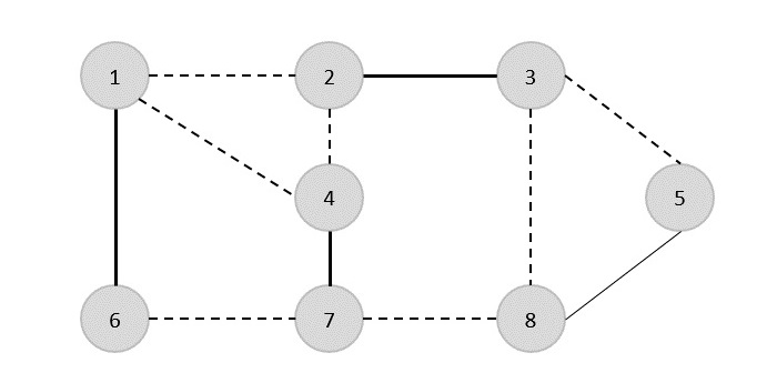
    Starting the algorithm from vertex 1, construct a minimum spanning tree from the graph. To learn more about constructing a minimum spanning tree, please click here.

    constructing_minimum_spanning_tree

    Step 2

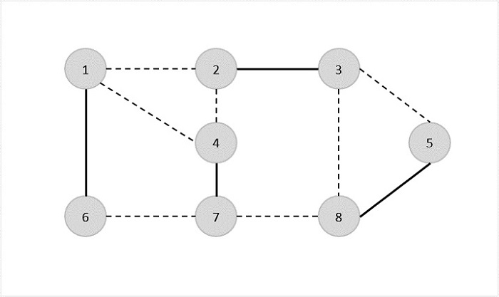
    Once, the minimum spanning tree is constructed, consider the starting vertex as the root node (i.e., vertex 1) and walk through the spanning tree preorderly.

    Rotating the spanning tree for easier interpretation, we get −

    Rotating_spanning_tree

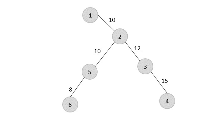
    The preorder traversal of the tree is found to be − 1 → 2 → 5 → 6 → 3 → 4

    Step 3

    Adding the root node at the end of the traced path, we get, 1 → 2 → 5 → 6 → 3 → 4 → 1

    This is the output Hamiltonian path of the travelling salesman approximation problem. The cost of the path would be the sum of all the costs in the minimum spanning tree, i.e., 55.

    Implementation

    Following are the implementations of the above approach in various programming langauges −

    CC++JavaPython

    #include <stdio.h>#include <stdbool.h>#include <limits.h>#define V 6 // Number of vertices in the graph// Function to find the minimum key vertex from the set of vertices not yet included in MSTintfindMinKey(int key[], bool mstSet[]){int min = INT_MAX, min_index;for(int v =0; v < V; v++){if(mstSet[v]== false && key[v]< min){
             min = key[v];
             min_index = v;}}return min_index;}// Function to perform Prim's algorithm to find the Minimum Spanning Tree (MST)voidprimMST(int graph[V][V],int parent[]){int key[V];
       bool mstSet[V];for(int i =0; i < V; i++){
          key[i]= INT_MAX;
          mstSet[i]= false;}
       key[0]=0;
       parent[0]=-1;for(int count =0; count < V -1; count++){int u =findMinKey(key, mstSet);
          mstSet[u]= true;for(int v =0; v < V; v++){if(graph[u][v]&& mstSet[v]== false && graph[u][v]< key[v]){
                parent[v]= u;
                key[v]= graph[u][v];}}}}// Function to print the preorder traversal of the Minimum Spanning TreevoidprintPreorderTraversal(int parent[]){printf("The preorder traversal of the tree is found to be  ");for(int i =1; i < V; i++){printf("%d  ", parent[i]);}printf("\n");}// Main function for the Traveling Salesperson Approximation AlgorithmvoidtspApproximation(int graph[V][V]){int parent[V];int root =0;// Choosing vertex 0 as the starting and ending point// Find the Minimum Spanning Tree using Prim's AlgorithmprimMST(graph, parent);// Print the preorder traversal of the Minimum Spanning TreeprintPreorderTraversal(parent);// Print the Hamiltonian path (preorder traversal with the starting point added at the end)printf("Adding the root node at the end of the traced path ");for(int i =0; i < V; i++){printf("%d  ", parent[i]);}printf("%d  %d\n", root, parent[0]);// Calculate and print the cost of the Hamiltonian pathint cost =0;for(int i =1; i < V; i++){
          cost += graph[parent[i]][i];}// The cost of the path would be the sum of all the costs in the minimum spanning tree.printf("Sum of all the costs in the minimum spanning tree %d.\n", cost);}intmain(){// Example graph represented as an adjacency matrixint graph[V][V]={{0,3,1,6,0,0},{3,0,5,0,3,0},{1,5,0,5,6,4},{6,0,5,0,0,2},{0,3,6,0,0,6},{0,0,4,2,6,0}};tspApproximation(graph);return0;}

    Output

    The preorder traversal of the tree is found to be  0  0  5  1  2  
    Adding the root node at the end of the traced path -1  0  0  5  1  2  0  -1
    Sum of all the costs in the minimum spanning tree 13.
  • Set Cover Problem

    The set cover algorithm provides solution to many real-world resource allocating problems. For instance, consider an airline assigning crew members to each of their airplanes such that they have enough people to fulfill the requirements for the journey. They take into account the flight timings, the duration, the pit-stops, availability of the crew to assign them to the flights. This is where set cover algorithm comes into picture.

    Given a universal set U, containing few elements which are all divided into subsets. Considering the collection of these subsets as S = {S1, S2, S3, S4… Sn}, the set cover algorithm finds the minimum number of subsets such that they cover all the elements present in the universal set.

    universal_set

    As shown in the above diagram, the dots represent the elements present in the universal set U that are divided into different sets, S = {S1, S2, S3, S4, S5, S6}. The minimum number of sets that need to be selected to cover all the elements will be the optimal output = {S1, S2, S3}.

    Set Cover Algorithm

    The set cover takes the collection of sets as an input and and returns the minimum number of sets required to include all the universal elements.

    The set cover algorithm is an NP-Hard problem and a 2-approximation greedy algorithm.

    Algorithm

    Step 1 − Initialize Output = {} where Output represents the output set of elements.

    Step 2 − While the Output set does not include all the elements in the universal set, do the following −

    • Find the cost-effectiveness of every subset present in the universal set using the formula, Cost(Si)Si−Output
    • Find the subset with minimum cost effectiveness for each iteration performed. Add the subset to the Output set.

    Step 3 − Repeat Step 2 until there is no elements left in the universe. The output achieved is the final Output set.

    Pseudocode

    APPROX-GREEDY-SET_COVER(X, S)
       U = X
       OUTPUT = 
       while U  
          select Si  S which has maximum |SiU|
       U = U  S
       OUTPUT = OUTPUT {Si}
    return OUTPUT
    

    Analysis

    assuming the overall number of elements equals the overall number of sets (|X| = |S|), the code runs in time O(|X|3)

    Example

    Set_Cover_Algorithm

    Let us look at an example that describes the approximation algorithm for the set covering problem in more detail

    S1 = {1, 2, 3, 4}                cost(S1) = 5
    S2 = {2, 4, 5, 8, 10}            cost(S2) = 10
    S3 = {1, 3, 5, 7, 9, 11, 13}     cost(S3) = 20
    S4 = {4, 8, 12, 16, 20}          cost(S4) = 12
    S5 = {5, 6, 7, 8, 9}             cost(S5) = 15
    

    Step 1

    The output set, Output =

    Find the cost effectiveness of each set for no elements in the output set,

    S1 = cost(S1) / (S1  Output) = 5 / (4  0)
    S2 = cost(S2) / (S2  Output) = 10 / (5  0)
    S3 = cost(S3) / (S3  Output) = 20 / (7  0)
    S4 = cost(S4) / (S4  Output) = 12 / (5  0)
    S5 = cost(S5) / (S5  Output) = 15 / (5  0)
    

    The minimum cost effectiveness in this iteration is achieved at S1, therefore, the subset added to the output set, Output = {S1} with elements {1, 2, 3, 4}

    Step 2

    Find the cost effectiveness of each set for the new elements in the output set,

    S2 = cost(S2) / (S2  Output) = 10 / (5  4)
    S3 = cost(S3) / (S3  Output) = 20 / (7  4)
    S4 = cost(S4) / (S4  Output) = 12 / (5  4)
    S5 = cost(S5) / (S5  Output) = 15 / (5  4)
    

    The minimum cost effectiveness in this iteration is achieved at S3, therefore, the subset added to the output set, Output = {S1, S3} with elements {1, 2, 3, 4, 5, 7, 9, 11, 13}.

    Step 3

    Find the cost effectiveness of each set for the new elements in the output set,

    S2 = cost(S2) / (S2  Output) = 10 / |(5  9)|
    S4 = cost(S4) / (S4  Output) = 12 / |(5  9)|
    S5 = cost(S5) / (S5  Output) = 15 / |(5  9)|
    

    The minimum cost effectiveness in this iteration is achieved at S2, therefore, the subset added to the output set, Output = {S1, S3, S2} with elements {1, 2, 3, 4, 5, 7, 8, 9, 10, 11, 13}

    Step 4

    Find the cost effectiveness of each set for the new elements in the output set,

    S4 = cost(S4) / (S4  Output) = 12 / |(5  11)|
    S5 = cost(S5) / (S5  Output) = 15 / |(5  11)|
    

    The minimum cost effectiveness in this iteration is achieved at S4, therefore, the subset added to the output set, Output = {S1, S3, S2, S4} with elements {1, 2, 3, 4, 5, 7, 8, 9, 10, 11, 12, 13, 16, 20}

    Step 5

    Find the cost effectiveness of each set for the new elements in the output set,

    S5 = cost(S5) / (S5  Output) = 15 / |(5  14)|
    

    The minimum cost effectiveness in this iteration is achieved at S5, therefore, the subset added to the output set, Output = {S1, S3, S2, S4, S5} with elements {1, 2, 3, 4, 5, 6, 7, 8, 9, 10, 11, 12, 13, 16, 20}

    The final output that covers all the elements present in the universal finite set is, Output = {S1, S3, S2, S4, S5}.

    Implementation

    Following are the implementations of the above approach in various programming langauges −

    CC++JavaPython

    #include <stdio.h>#define MAX_SETS 100#define MAX_ELEMENTS 1000intsetCover(int X[],int S[][MAX_ELEMENTS],int numSets,int numElements,int output[]){int U[MAX_ELEMENTS];for(int i =0; i < numElements; i++){
          U[i]= X[i];}int selectedSets[MAX_SETS];for(int i =0; i < MAX_SETS; i++){
          selectedSets[i]=0;// Initialize all to 0 (not selected)}int outputIdx =0;while(outputIdx < numSets){// Ensure we don't exceed the maximum number of setsint maxIntersectionSize =0;int selectedSetIdx =-1;// Find the set Si with the maximum intersection with Ufor(int i =0; i < numSets; i++){if(selectedSets[i]==0){// Check if the set is not already selectedint intersectionSize =0;for(int j =0; j < numElements; j++){if(U[j]&& S[i][j]){
                      intersectionSize++;}}if(intersectionSize > maxIntersectionSize){
                   maxIntersectionSize = intersectionSize;
                   selectedSetIdx = i;}}}// If no set found, break from the loopif(selectedSetIdx ==-1){break;}// Mark the selected set as "selected" in the array
          selectedSets[selectedSetIdx]=1;// Remove the elements covered by the selected set from Ufor(int j =0; j < numElements; j++){
              U[j]= U[j]- S[selectedSetIdx][j];}// Add the selected set to the output
          output[outputIdx++]= selectedSetIdx;}return outputIdx;}intmain(){int X[MAX_ELEMENTS]={1,2,3,4,5,6,7,8,9,10};int S[MAX_SETS][MAX_ELEMENTS]={{1,1,0,0,0,0,0,0,0,0},{0,1,1,1,0,0,0,0,0,0},{0,0,0,1,1,1,0,0,0,0},{0,0,0,0,0,1,1,1,0,0},{0,0,0,0,0,0,0,1,1,1}};int numSets =5;int numElements =10;int output[MAX_SETS];int numSelectedSets =setCover(X, S, numSets, numElements, output);printf("Selected Sets: ");for(int i =0; i < numSelectedSets; i++){printf("%d ", output[i]);}printf("\n");return0;}

    Output

    Selected Sets: 1 2 3 4 0
  • Vertex Cover Algorithm

    Have you ever wondered about the placement of traffic cameras? That how they are efficiently placed without wasting too much budget from the government? The answer to that comes in the form of vertex-cover algorithm. The positions of the cameras are chosen in such a way that one camera covers as many roads as possible, i.e., we choose junctions and make sure the camera covers as much area as possible.

    vertex-cover of an undirected graph G = (V,E) is the subset of vertices of the graph such that, for all the edges (u,v) in the graph,u and v ∈ V. The junction is treated as the node of a graph and the roads as the edges. The algorithm finds the minimum set of junctions that cover maximum number of roads.

    It is a minimization problem since we find the minimum size of the vertex cover the size of the vertex cover is the number of vertices in it. The optimization problem is an NP-Complete problem and hence, cannot be solved in polynomial time; but what can be found in polynomial time is the near optimal solution.

    Vertex Cover Algorithm

    The vertex cover approximation algorithm takes an undirected graph as an input and is executed to obtain a set of vertices that is definitely twice as the size of optimal vertex cover.

    The vertex cover is a 2-approximation algorithm.

    Algorithm

    Step 1 − Select any random edge from the input graph and mark all the edges that are incident on the vertices corresponding to the selected edge.

    Step 2 − Add the vertices of the arbitrary edge to an output set.

    Step 3 − Repeat Step 1 on the remaining unmarked edges of the graph and add the vertices chosen to the output until theres no edge left unmarked.

    Step 4 − The final output set achieved would be the near-optimal vertex cover.

    Pseudocode

    APPROX-VERTEX_COVER (G: Graph)
    c ← { }
    E ← E[G]
    while E is not empty do
       Let (u, v) be an arbitrary edge of E
       c ← c U {u, v}
       Remove from E every edge incident on either u or v
    return c
    

    Example

    The set of edges of the given graph is −

    {(1,6),(1,2),(1,4),(2,3),(2,4),(6,7),(4,7),(7,8),(3,5),(8,5)}
    
    Vertex_Cover_Problem

    Now, we start by selecting an arbitrary edge (1,6). We eliminate all the edges, which are either incident to vertex 1 or 6 and we add edge (1,6) to cover.

    arbitrary_edge

    In the next step, we have chosen another edge (2,3) at random.

    chosen_another_edge

    Now we select another edge (4,7).

    select_another_edge

    We select another edge (8,5).

    another edge 8 to 5

    Hence, the vertex cover of this graph is {1,6,2,3,4,7,5,8}.

    Analysis

    It is easy to see that the running time of this algorithm is O(V + E), using adjacency list to represent E’.

    Implementation

    Following are the implementations of the above approach in various programming langauges −

    CC++JavaPython

    #include <stdio.h>#include <stdbool.h>#define MAX_VERTICES 100int graph[MAX_VERTICES][MAX_VERTICES];
    bool included[MAX_VERTICES];// Function to find Vertex Cover using the APPROX-VERTEX_COVER algorithmvoidapproxVertexCover(int vertices,int edges){
       bool edgesRemaining[MAX_VERTICES][MAX_VERTICES];for(int i =0; i < vertices; i++){for(int j =0; j < vertices; j++){
             edgesRemaining[i][j]= graph[i][j];}}while(edges >0){int u, v;for(int i =0; i < vertices; i++){for(int j =0; j < vertices; j++){if(edgesRemaining[i][j]){
                   u = i;
                   v = j;break;}}}
          included[u]= included[v]= true;for(int i =0; i < vertices; i++){
             edgesRemaining[u][i]= edgesRemaining[i][u]= false;
             edgesRemaining[v][i]= edgesRemaining[i][v]= false;}
          edges--;}}intmain(){int vertices =8;int edges =10;int edgesData[10][2]={{1,6},{1,2},{1,4},{2,3},{2,4},{6,7},{4,7},{7,8},{3,5},{8,5}};for(int i =0; i < edges; i++){int u = edgesData[i][0];int v = edgesData[i][1];
          graph[u][v]= graph[v][u]=1;}approxVertexCover(vertices, edges);printf("Vertex Cover: ");for(int i =1; i <= vertices; i++){if(included[i]){printf("%d ", i);}}printf("\n");return0;}

    Output

    Vertex Cover: 1 3 4 5 6 7 
  • Approximation Algorithms

    Approximation Algorithms

    Approximation algorithms are algorithms designed to solve problems that are not solvable in polynomial time for approximate solutions. These problems are known as NP complete problems. These problems are significantly effective to solve real world problems, therefore, it becomes important to solve them using a different approach.

    NP complete problems can still be solved in three cases: the input could be so small that the execution time is reduced, some problems can still be classified into problems that can be solved in polynomial time, or use approximation algorithms to find near-optima solutions for the problems.

    This leads to the concept of performance ratios of an approximation problem.

    Performance Ratios

    The main idea behind calculating the performance ratio of an approximation algorithm, which is also called as an approximation ratio, is to find how close the approximate solution is to the optimal solution.

    The approximate ratio is represented using (n) where n is the input size of the algorithm, C is the near-optimal solution obtained by the algorithm, C* is the optimal solution for the problem. The algorithm has an approximate ratio of (n) if and only if −

    max{CC∗,C∗C}≤ρ(n)

    The algorithm is then called a (n)-approximation algorithm. Approximation Algorithms can be applied on two types of optimization problems: minimization problems and maximization problems. If the optimal solution of the problem is to find the maximum cost, the problem is known as the maximization problem; and if the optimal solution of the problem is to find the minimum cost, then the problem is known as a minimization problem.

    For maximization problems, the approximation ratio is calculated by C*/C since 0 C C*. For minimization problems, the approximation ratio is calculated by C/C* since 0 C* C.

    Assuming that the costs of approximation algorithms are all positive, the performance ratio is well defined and will not be less than 1. If the value is 1, that means the approximate algorithm generates the exact optimal solution.

    Examples

    Few popular examples of the approximation algorithms are −

    • Vertex Cover Algorithm
    • Set Cover Problem
    • Travelling Salesman Problem (Approximation Approach)
    • The Subset Sum Problem