Author: admin

  • Radix Sort Algorithm

    Radix sort is a step-wise sorting algorithm that starts the sorting from the least significant digit of the input elements. Like Counting Sort and Bucket Sort, Radix sort also assumes something about the input elements, that they are all k-digit numbers.

    The sorting starts with the least significant digit of each element. These least significant digits are all considered individual elements and sorted first; followed by the second least significant digits. This process is continued until all the digits of the input elements are sorted.

    Note − If the elements do not have same number of digits, find the maximum number of digits in an input element and add leading zeroes to the elements having less digits. It does not change the values of the elements but still makes them k-digit numbers.

    Radix Sort Algorithm

    The radix sort algorithm makes use of the counting sort algorithm while sorting in every phase. The detailed steps are as follows −

    Step 1 − Check whether all the input elements have same number of digits. If not, check for numbers that have maximum number of digits in the list and add leading zeroes to the ones that do not.

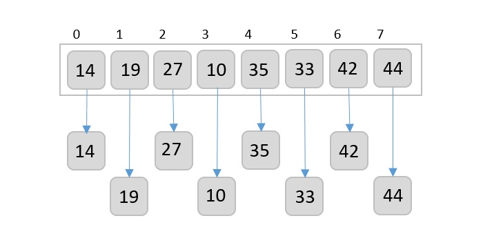
    Step 2 − Take the least significant digit of each element.

    Step 3 − Sort these digits using counting sort logic and change the order of elements based on the output achieved. For example, if the input elements are decimal numbers, the possible values each digit can take would be 0-9, so index the digits based on these values.

    Step 4 − Repeat the Step 2 for the next least significant digits until all the digits in the elements are sorted.

    Step 5 − The final list of elements achieved after kth loop is the sorted output.

    Pseudocode

    Algorithm: RadixSort(a[], n):
       
       // Find the maximum element of the list
       max = a[0]
       for (i=1 to n-1):
          if (a[i]>max):
             max=a[i]
    
       // applying counting sort for each digit in each number of 
       //the input list
       For (pos=1 to max/pos>0):
          countSort(a, n, pos)
          pos=pos*10
    

    The countSort algorithm called would be −

    Algorithm: countSort(a, n, pos)
       Initialize count[09] with zeroes
       for i = 0 to n:
          count[(a[i]/pos) % 10]++
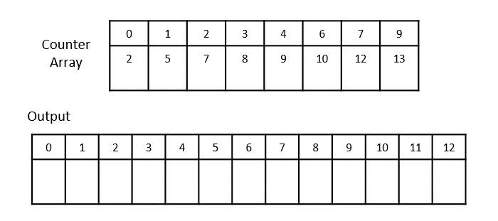
       for i = 1 to 10:
          count[i] = count[i] + count[i-1]
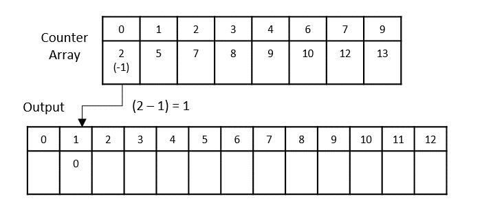
       for i = n-1 to 0:
          output[count[(a[i]/pos) % 10]-1] = a[i]
          i--
       for i to n:
          a[i] = output[i]
    

    Analysis

    Given that there are k-digits in the input elements, the running time taken by the radix sort algorithm would be Θ(k(n + b). Here, n is the number of elements in the input list while b is the number of possible values each digit of a number can take.

    Example

    For the given unsorted list of elements, 236, 143, 26, 42, 1, 99, 765, 482, 3, 56, we need to perform the radix sort and obtain the sorted output list −

    Step 1

    Check for elements with maximum number of digits, which is 3. So we add leading zeroes to the numbers that do not have 3 digits. The list we achieved would be −

    236, 143, 026, 042, 001, 099, 765, 482, 003, 056
    

    Step 2

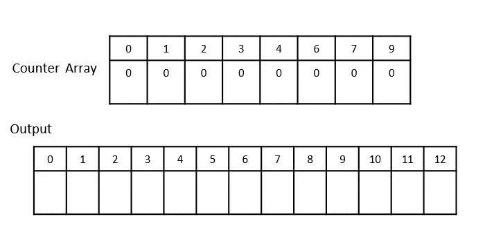
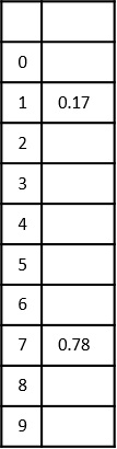
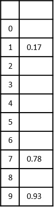
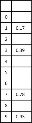
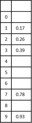
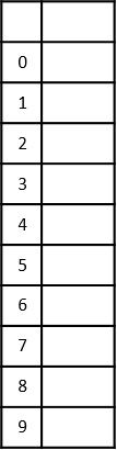
    Construct a table to store the values based on their indexing. Since the inputs given are decimal numbers, the indexing is done based on the possible values of these digits, i.e., 0-9.

    Construct_table

    Step 3

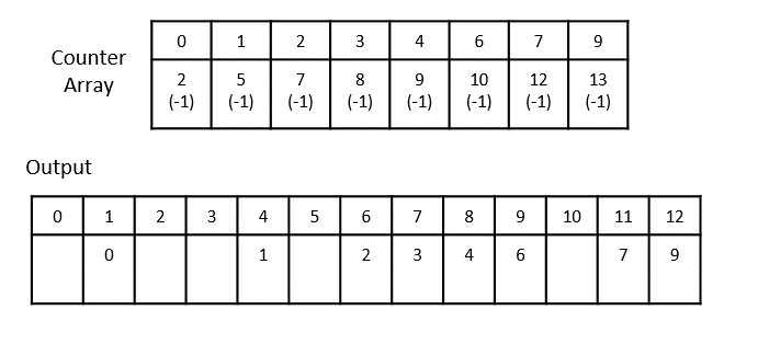
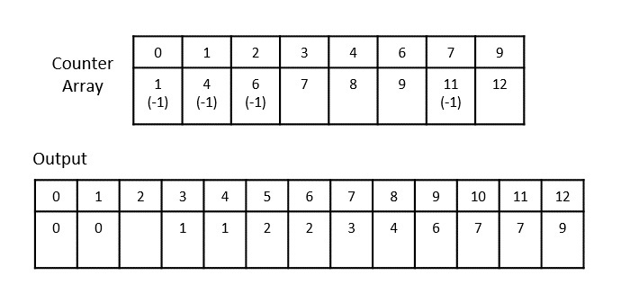
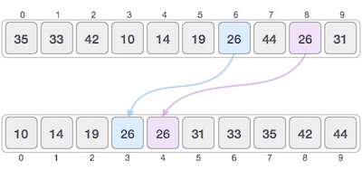
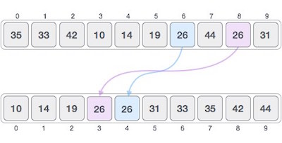
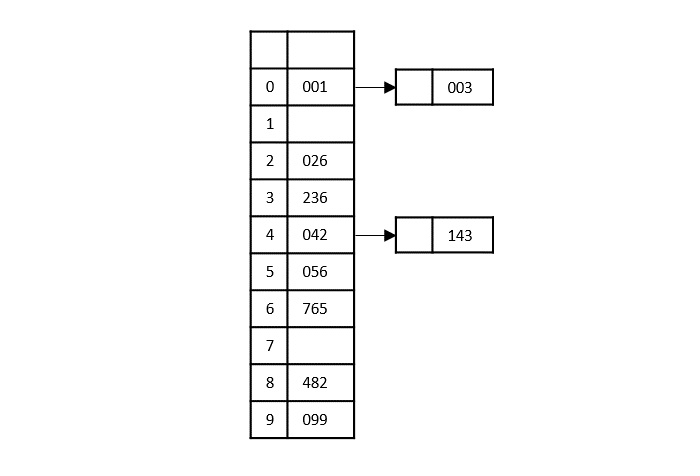
    Based on the least significant digit of all the numbers, place the numbers on their respective indices.

    least_significant_digit

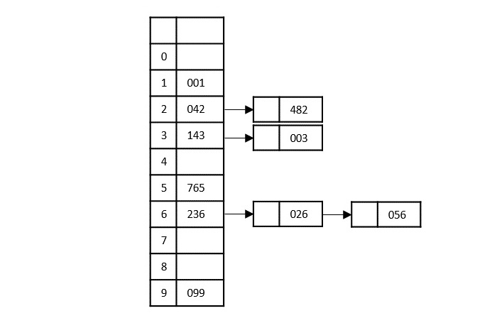
    The elements sorted after this step would be 001, 042, 482, 143, 003, 765, 236, 026, 056, 099.

    Step 4

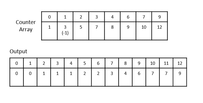
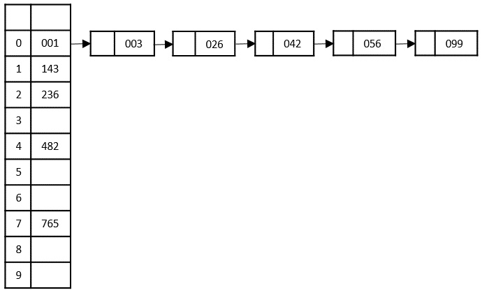
    The order of input for this step would be the order of the output in the previous step. Now, we perform sorting using the second least significant digit.

    second_least_significant_digit

    The order of the output achieved is 001, 003, 026, 236, 042, 143, 056, 765, 482, 099.

    Step 5

    The input list after the previous step is rearranged as −

    001, 003, 026, 236, 042, 143, 056, 765, 482, 099
    

    Now, we need to sort the last digits of the input elements.

    last_digits

    Since there are no further digits in the input elements, the output achieved in this step is considered as the final output.

    The final sorted output is −

    1, 3, 26, 42, 56, 99, 143, 236, 482, 765
    

    Implementation

    The counting sort algorithm assists the radix sort to perform sorting on multiple d-digit numbers iteratively for d loops. Radix sort is implemented in four programming languages in this tutorial: C, C++, Java, Python.

    CC++JavaPython

    #include <stdio.h>voidcountsort(int a[],int n,int pos){int output[n +1];int max =(a[0]/ pos)%10;for(int i =1; i < n; i++){if(((a[i]/ pos)%10)> max)
             max = a[i];}int count[max +1];for(int i =0; i < max;++i)
          count[i]=0;for(int i =0; i < n; i++)
          count[(a[i]/ pos)%10]++;for(int i =1; i <10; i++)
          count[i]+= count[i -1];for(int i = n -1; i >=0; i--){
          output[count[(a[i]/ pos)%10]-1]= a[i];
          count[(a[i]/ pos)%10]--;}for(int i =0; i < n; i++)
          a[i]= output[i];}voidradixsort(int a[],int n){int max = a[0];for(int i =1; i < n; i++)if(a[i]> max)
             max = a[i];for(int pos =1; max / pos >0; pos *=10)countsort(a, n, pos);}intmain(){int a[]={236,15,333,27,9,108,76,498};int n =sizeof(a)/sizeof(a[0]);printf("Before sorting array elements are: ");for(int i =0; i <n;++i){printf("%d ", a[i]);}radixsort(a, n);printf("\nAfter sorting array elements are: ");for(int i =0; i < n;++i){printf("%d ", a[i]);}printf("\n");}

    Output

    Before sorting array elements are: 236 15 333 27 9 108 76 498 
    After sorting array elements are: 9 15 27 76 108 236 333 498
  • Counting Sort Algorithm

    Counting sort is an external sorting algorithm that assumes all the input values are integers that lie between the range 0 and k. Then mathematical computations on these input values to place them at the correct position in the output array.

    This algorithm makes use of a counter to count the frequency of occurrence of the numbers and arrange them accordingly. Suppose, if a number m occurs 5 times in the input sequence, the counter value of the number will become 5 and it is repeated 5 times in the output array.

    Counting Sort Algorithm

    The counting sort algorithm assumes that the input is relatively smaller so the algorithm is as follows −

    Step 1 − Maintain two arrays, one with the size of input elements without repetition to store the count values and other with the size of the input array to store the output.

    Step 2 − Initialize the count array with all zeroes and keep the output array empty.

    Step 3 − Every time an element occurs in the input list, increment the corresponding counter value by 1, until it reaches the end of the input list.

    Step 4 − Now, in the output array, every time a counter is greater than 0, add the element at its respective index, i.e. if the counter of 0 is 2, 0 added at the 2nd position (i.e. 1st index) of the output array. Then decrement the counter value by 1.

    Step 5 − Repeat Step 4 until all the counter values become 0. The list obtained is the output list.

    COUNTING-SORT(A, B, k)
    let C[0  k] be a new array
    for i = 0 to k
    C[i] = 0
    for j = 1 to A.length
    C[A[j]] = C[A[j]] + 1
    
    // C[i] now contains the number of elements equal to i.
    for i = 1 to k
    C[i] = C[i] + C[i  1]
    // C[i] now contains the number of elements less than or equal to i.
    for j = A.length downto 1
    B[C[A[j]]] = A[j]
    C[A[j]] = C[A[j  1]
    

    Analysis

    The average case time complexity for the counting sort algorithm is same as bucket sort. It runs in (n) time.

    Example

    Consider an input list to be sorted, 0, 2, 1, 4, 6, 2, 1, 1, 0, 3, 7, 7, 9.

    For easier computations, let us start with single digit numbers.

    Step 1

    Create two arrays: to store counters and the output. Initialize the counter array with zeroes.

    create_two_arrays

    Step 2

    After incrementing all the counter values until it reaches the end of the input list, we achieve −

    incrementing_all_counter

    Step 3

    Now, push the elements at the corresponding index in the output list.

    push_elements

    Step 4

    Decrement the counter by 1 after adding the elements in the output array. Now, 1 is added at the 4th index.

    Decrement_counter

    Step 5

    Add the remaining values preceding the index in previous step.

    Add_remaining_values

    Step 6

    After adding the last values, we get −

    adding_last_values

    The final sorted output is achieved as 0, 0, 1, 1, 1, 2, 2, 3, 4, 6, 7, 7, 9

    Implementation

    The counting sort implementation works closely with the algorithm where we construct an array to store the frequency of each element of the input array. Based on these frequencies, the elements are placed in the output array. Repetitive elements are also sorted in the counting sort algorithm.

    Example

    In this chapter, we look into the counting sort program implemented in four different programming languages.

    CC++JavaPython

    #include<stdio.h>intcountingsort(int a[],int n){int i, j;int output[15], c[100];for(i =0; i <100; i++)
          c[i]=0;for(j =0; j < n; j++)++c[a[j]];for(i =1; i <=99; i++)
          c[i]+= c[i-1];for(j = n-1; j >=0; j--){
          output[c[a[j]]-1]= a[j];--c[a[j]];}printf("\nAfter sorting array elements are: ");for(i =0; i<n; i++)printf("%d ", output[i]);}voidmain(){int n , i;int a[]={12,32,44,8,16};
       n =sizeof(a)/sizeof(a[0]);printf("Before sorting array elements are: ");for(int i =0; i<n; i++){printf("%d ", a[i]);}countingsort(a, n);}

    Output

    Before sorting array elements are: 12 32 44 8 16 
    After sorting array elements are: 8 12 16 32 44
  • Bucket Sort Algorithm

    The Bucket Sort algorithm is similar to the Counting Sort algorithm, as it is just the generalized form of the counting sort. Bucket sort assumes that the input elements are drawn from a uniform distribution over the interval [0, 1).

    Hence, the bucket sort algorithm divides the interval [0, 1) into n equal parts, and the input elements are added to indexed buckets where the indices based on the lower bound of the (n element) value. Since the algorithm assumes the values as the independent numbers evenly distributed over a small range, not many elements fall into one bucket only.

    For example, let us look at an input list of elements, 0.08, 0.01, 0.19, 0.89, 0.34, 0.07, 0.30, 0.82, 0.39, 0.45, 0.36. The bucket sort would look like −

    bucket_sort

    Bucket Sort Algorithm

    Let us look at how this algorithm would proceed further below −

    Step 1 − Divide the interval in n equal parts, each part being referred to as a bucket. Say if n is 10, then there are 10 buckets; otherwise more.

    Step 2 − Take the input elements from the input array A and add them to these output buckets B based on the computation formula, B[i]= ⌊n.A[i]⌋

    Step 3 − If there are any elements being added to the already occupied buckets, created a linked list through the corresponding bucket.

    Step 4 − Then we apply insertion sort to sort all the elements in each bucket.

    Step 5 − These buckets are concatenated together which in turn is obtained as the output.

    Pseudocode

    BUCKET-SORT(A)
    let B[0  n  1] be a new array
    n = A.length
    for i = 0 to n  1
       make B[i] an empty list
    for i = 1 to n
       insert A[i] into list B[$\lfloor$.[]$\rfloor$]
    for i = 0 to n  1
       sort list B[i] with insertion sort
    concatenate the lists B[0], B[1];  ; B[n  1] together in order
    

    Analysis

    The bucket sort algorithm assumes the identity of the input, therefore, the average case time complexity of the algorithm is (n)

    Example

    Consider, an input list of elements, 0.78, 0.17, 0.93, 0.39, 0.26, 0.72, 0.21, 0.12, 0.33, 0.28, to sort these elements using bucket sort −

    Solution

    Step 1

    Linearly insert all the elements from the index 0 of the input array. That is, we insert 0.78 first followed by other elements sequentially. The position to insert the element is obtained using the formula − B[i]= ⌊n.A[i]⌋, i.e, ⌊10 0.78⌋=7

    insert_element

    Now, we insert 0.17 at index ⌊10 0.17⌋=1

    insert_at_index_1

    Step 3

    Inserting the next element, 0.93 into the output buckets at ⌊10 0.93⌋=9

    insert_at_index_9

    Step 4

    Insert 0.39 at index 3 using the formula ⌊10 0.39⌋=3

    insert_at_index_3

    Step 5

    Inserting the next element in the input array, 0.26, at position ⌊10 0.26⌋=2

    insert_at_index_2

    Step 6

    Here is where it gets tricky. Now, the next element in the input list is 0.72 which needs to be inserted at index 7 using the formula ⌊10 0.72⌋=7. But theres already a number in the 7th bucket. So, a link is created from the 7th index to store the new number like a linked list, as shown below −

    insert_index_at_7_new_value

    Step 7

    Add the remaining numbers to the buckets in the similar manner by creating linked lists from the desired buckets. But while inserting these elements as lists, we apply insertion sort, i.e., compare the two elements and add the minimum value at the front as shown below −

    apply_insertion_sort

    Step 8

    Now, to achieve the output, concatenate all the buckets together.

    0.12, 0.17, 0.21, 0.26, 0.28, 0.33, 0.39, 0.72, 0.78, 0.93

    Implementation

    The implementation of the bucket sort algorithm first retrieves the maximum element of the array and decides the bucket size of the output. The elements are inserted into these buckets based on few computations.

    In this tutorial, we execute bucket sort in four programming languages.

    CC++JavaPython

    #include <stdio.h>voidbucketsort(int a[],int n){// function to implement bucket sortint max = a[0];// get the maximum element in the arrayfor(int i =1; i < n; i++)if(a[i]> max)
             max = a[i];int b[max], i;for(int i =0; i <= max; i++){
          b[i]=0;}for(int i =0; i < n; i++){
          b[a[i]]++;}for(int i =0, j =0; i <= max; i++){while(b[i]>0){
             a[j++]= i;
             b[i]--;}}}intmain(){int a[]={12,45,33,87,56,9,11,7,67};int n =sizeof(a)/sizeof(a[0]);// n is the size of arrayprintf("Before sorting array elements are: \n");for(int i =0; i < n;++i)printf("%d ", a[i]);bucketsort(a, n);printf("\nAfter sorting array elements are: \n");for(int i =0; i < n;++i)printf("%d ", a[i]);}

    Output

    Before sorting array elements are: 
    12 45 33 87 56 9 11 7 67 
    After sorting array elements are: 
    7 9 11 12 33 45 56 67 87
  • Heap Sort Algorithm

    Heap Sort is an efficient sorting technique based on the heap data structure.

    The heap is a nearly-complete binary tree where the parent node could either be minimum or maximum. The heap with minimum root node is called min-heap and the root node with maximum root node is called max-heap. The elements in the input data of the heap sort algorithm are processed using these two methods.

    The heap sort algorithm follows two main operations in this procedure −

    • Builds a heap H from the input data using the heapify (explained further into the chapter) method, based on the way of sorting ascending order or descending order.
    • Deletes the root element of the root element and repeats until all the input elements are processed.

    The heap sort algorithm heavily depends upon the heapify method of the binary tree. So what is this heapify method?

    Heapify Method

    The heapify method of a binary tree is to convert the tree into a heap data structure. This method uses recursion approach to heapify all the nodes of the binary tree.

    Note − The binary tree must always be a complete binary tree as it must have two children nodes always.

    The complete binary tree will be converted into either a max-heap or a min-heap by applying the heapify method.

    To know more about the heapify algorithm, please click here.

    Heap Sort Algorithm

    As described in the algorithm below, the sorting algorithm first constructs the heap ADT by calling the Build-Max-Heap algorithm and removes the root element to swap it with the minimum valued node at the leaf. Then the heapify method is applied to rearrange the elements accordingly.

    Algorithm: Heapsort(A)
    BUILD-MAX-HEAP(A)
    for i = A.length downto 2
    exchange A[1] with A[i]
    A.heap-size = A.heap-size - 1
    MAX-HEAPIFY(A, 1)
    

    Analysis

    The heap sort algorithm is the combination of two other sorting algorithms: insertion sort and merge sort.

    The similarities with insertion sort include that only a constant number of array elements are stored outside the input array at any time.

    The time complexity of the heap sort algorithm is O(nlogn), similar to merge sort.

    Example

    Let us look at an example array to understand the sort algorithm better −

    1239141018823

    Building a heap using the BUILD-MAX-HEAP algorithm from the input array −

    build_max_heap

    Rearrange the obtained binary tree by exchanging the nodes such that a heap data structure is formed.

    heap_data_structure
    23_to_3
    23_to_12
    14_to_3
    14_to_12
    18_to_9.jpg

    The Heapify Algorithm

    Applying the heapify method, remove the root node from the heap and replace it with the next immediate maximum valued child of the root.

    The root node is 23, so 23 is popped and 18 is made the next root because it is the next maximum node in the heap.

    23_popped

    Now, 18 is popped after 23 which is replaced by 14.

    18_popped

    The current root 14 is popped from the heap and is replaced by 12.

    14_popped

    12 is popped and replaced with 10.

    12_popped

    Similarly all the other elements are popped using the same process.

    10_popped

    Here the current root element 9 is popped and the elements 8 and 3 are remained in the tree.

    9_popped

    Then, 8 will be popped leaving 3 in the tree.

    8_popped.jpg

    After completing the heap sort operation on the given heap, the sorted elements are displayed as shown below −

    all_element_popped.jpg

    Every time an element is popped, it is added at the beginning of the output array since the heap data structure formed is a max-heap. But if the heapify method converts the binary tree to the min-heap, add the popped elements are on the end of the output array.

    The final sorted list is,

    3891012141823

    Implementation

    The logic applied on the implementation of the heap sort is: firstly, the heap data structure is built based on the max-heap property where the parent nodes must have greater values than the child nodes. Then the root node is popped from the heap and the next maximum node on the heap is shifted to the root. The process is continued iteratively until the heap is empty.

    In this tutorial, we show the heap sort implementation in four different programming languages.

    CC++JavaPython

    #include <stdio.h>voidheapify(int[],int);voidbuild_maxheap(int heap[],int n){int i, j, c, r, t;for(i =1; i < n; i++){
          c = i;do{
             r =(c -1)/2;if(heap[r]< heap[c]){// to create MAX heap array
                t = heap[r];
                heap[r]= heap[c];
                heap[c]= t;}
             c = r;}while(c !=0);}printf("Heap array: ");for(i =0; i < n; i++)printf("%d ", heap[i]);heapify(heap, n);}voidheapify(int heap[],int n){int i, j, c, root, temp;for(j = n -1; j >=0; j--){
          temp = heap[0];
          heap[0]= heap[j];// swap max element with rightmost leaf element
          heap[j]= temp;
          root =0;do{
             c =2* root +1;// left node of root elementif((heap[c]< heap[c +1])&& c < j-1)
                c++;if(heap[root]<heap[c]&& c<j){// again rearrange to max heap array
                temp = heap[root];
                heap[root]= heap[c];
                heap[c]= temp;}
             root = c;}while(c < j);}printf("\nThe sorted array is: ");for(i =0; i < n; i++)printf("%d ", heap[i]);}intmain(){int n, i, j, c, root, temp;
       n =5;int heap[10]={2,3,1,0,4};// initialize the arraybuild_maxheap(heap, n);}

    Output

    Heap array: 4 3 1 0 2 
    The sorted array is: 0 1 2 3 4 
  • Shell Sort Algorithm

    Shell sort is a highly efficient sorting algorithm and is based on insertion sort algorithm. This algorithm avoids large shifts as in case of insertion sort, if the smaller value is to the far right and has to be moved to the far left.

    This algorithm uses insertion sort on a widely spread elements, first to sort them and then sorts the less widely spaced elements. This spacing is termed as interval. This interval is calculated based on Knuth’s formula as −

    h = h * 3 + 1
    where 
       h is interval with initial value 1
    

    This algorithm is quite efficient for medium-sized data sets as its average and worst case complexity are of O(n), where n is the number of items.

    Shell Sort Algorithm

    Following is the algorithm for shell sort.

    1. Initialize the value of h.
    2. Divide the list into smaller sub-list of equal interval h.
    3. Sort these sub-lists using insertion sort.
    4. Repeat until complete list is sorted.
    

    Pseudocode

    Following is the pseudocode for shell sort.

    procedure shellSort()
       A : array of items
    
       /* calculate interval*/
       while interval < A.length /3 do:
          interval = interval * 3 + 1
       end while
    
       while interval > 0 do:
          for outer = interval; outer < A.length; outer ++ do:
    
             /* select value to be inserted */
             valueToInsert = A[outer]
             inner = outer;
                
                /*shift element towards right*/
                while inner > interval -1 &&  A[inner - interval] 
    			>= valueToInsert do:
                   A[inner] = A[inner - interval]
                   inner = inner  interval
                end while
             
             /* insert the number at hole position */
             A[inner] = valueToInsert
             end for
       
       /* calculate interval*/
       interval = (interval -1) /3;
       end while
    end procedure
    

    Example

    Let us consider the following example to have an idea of how shell sort works. We take the same array we have used in our previous examples. For our example and ease of understanding, we take the interval of 4. Make a virtual sub-list of all values located at the interval of 4 positions. Here these values are {35, 14}, {33, 19}, {42, 27} and {10, 14}

    shell_sort_works

    We compare values in each sub-list and swap them (if necessary) in the original array. After this step, the new array should look like this −

    compare_values

    Then, we take interval of 2 and this gap generates two sub-lists – {14, 27, 35, 42}, {19, 10, 33, 44}

    two_sub_lists

    We compare and swap the values, if required, in the original array. After this step, the array should look like this −

    compare_values

    Finally, we sort the rest of the array using interval of value 1. Shell sort uses insertion sort to sort the array.

    Following is the step-by-step depiction −

    step-by-step
    step-by-step_depiction
    repalce_19_to_27
    replace_10_with_27
    replaced_27_with_10
    replace_10_19
    replace_10_14
    replace_values_sorted
    replace_33_35
    replaced_33_with_35
    choose_44
    sorted_array

    We see that it required only four swaps to sort the rest of the array.

    Implementation

    Shell sort is a highly efficient sorting algorithm and is based on insertion sort algorithm. This algorithm avoids large shifts as in case of insertion sort, if the smaller value is to the far right and has to be moved to the far left.

    CC++JavaPython

    #include <stdio.h>voidshellSort(int arr[],int n){int gap, j, k;for(gap = n/2; gap >0; gap = gap /2){//initially gap = n/2, decreasing by gap /2for(j = gap; j<n; j++){for(k = j-gap; k>=0; k -= gap){if(arr[k+gap]>= arr[k])break;else{int temp;
                   temp = arr[k+gap];
                   arr[k+gap]= arr[k];
                   arr[k]= temp;}}}}}intmain(){int n;
       n =5;int arr[5]={33,45,62,12,98};// initialize the arrayprintf("Array before Sorting: ");for(int i =0; i<n; i++)printf("%d ",arr[i]);printf("\n");shellSort(arr, n);printf("Array after Sorting: ");for(int i =0; i<n; i++)printf("%d ", arr[i]);printf("\n");}

    Output

    Array before Sorting: 33 45 62 12 98
    Array after Sorting: 12 33 45 62 98
  • Merge Sort Algorithm

    Merge sort is a sorting technique based on divide and conquer technique. With worst-case time complexity being (n log n), it is one of the most used and approached algorithms.

    Merge sort first divides the array into equal halves and then combines them in a sorted manner.

    How Merge Sort Works?

    To understand merge sort, we take an unsorted array as the following −

    unsorted array

    We know that merge sort first divides the whole array iteratively into equal halves unless the atomic values are achieved. We see here that an array of 8 items is divided into two arrays of size 4.

    divides array

    This does not change the sequence of appearance of items in the original. Now we divide these two arrays into halves.

    two arrays into halves

    We further divide these arrays and we achieve atomic value which can no more be divided.

    atomic value

    Now, we combine them in exactly the same manner as they were broken down. Please note the color codes given to these lists.

    We first compare the element for each list and then combine them into another list in a sorted manner. We see that 14 and 33 are in sorted positions. We compare 27 and 10 and in the target list of 2 values we put 10 first, followed by 27. We change the order of 19 and 35 whereas 42 and 44 are placed sequentially.

    compare element

    In the next iteration of the combining phase, we compare lists of two data values, and merge them into a list of found data values placing all in a sorted order.

    sorted order

    After the final merging, the list becomes sorted and is considered the final solution.

    merge sort

    Merge Sort Algorithm

    Merge sort keeps on dividing the list into equal halves until it can no more be divided. By definition, if it is only one element in the list, it is considered sorted. Then, merge sort combines the smaller sorted lists keeping the new list sorted too.

    Step 1: If it is only one element in the list, consider it already 
    sorted, so return.
    Step 2: Divide the list recursively into two halves until it can no  
    more be divided.
    Step 3: Merge the smaller lists into new list in sorted order.
    

    Pseudocode

    We shall now see the pseudocodes for merge sort functions. As our algorithms point out two main functions divide & merge.

    Merge sort works with recursion and we shall see our implementation in the same way.

    procedure mergesort( var a as array )
       if ( n == 1 ) return a
          var l1 as array = a[0] ... a[n/2]
          var l2 as array = a[n/2+1] ... a[n]
          l1 = mergesort( l1 )
          l2 = mergesort( l2 )
          return merge( l1, l2 )
    end procedure
    procedure merge( var a as array, var b as array )
       var c as array
       while ( a and b have elements )
          if ( a[0] > b[0] )
             add b[0] to the end of c
             remove b[0] from b
          else
             add a[0] to the end of c
             remove a[0] from a
          end if
       end while
       while ( a has elements )
          add a[0] to the end of c
          remove a[0] from a
       end while
       while ( b has elements )
          add b[0] to the end of c
          remove b[0] from b
       end while
       return c
    end procedure
    

    Example

    In the following example, we have shown Merge-Sort algorithm step by step. First, every iteration array is divided into two sub-arrays, until the sub-array contains only one element. When these sub-arrays cannot be divided further, then merge operations are performed.

    Merge Sort algorithm

    Analysis

    Let us consider, the running time of Merge-Sort as T(n). Hence,

    T(n)={c2xT(n2)+dxnifn≤1otherwisewherecanddareconstants

    Therefore, using this recurrence relation,

    T(n)=2iT(n/2i)+i⋅d⋅n

    As,i=logn,T(n)=2lognT(n/2logn)+logn⋅d⋅n

    =c⋅n+d⋅n⋅logn

    Therefore,T(n)=O(nlogn).

    Example

    Following are the implementations of the above approach in various programming languages −

    CC++JavaPython

    #include <stdio.h>#define max 10int a[11]={10,14,19,26,27,31,33,35,42,44,0};int b[10];voidmerging(int low,int mid,int high){int l1, l2, i;for(l1 = low, l2 = mid +1, i = low; l1 <= mid && l2 <= high; i++){if(a[l1]<= a[l2])
             b[i]= a[l1++];else
             b[i]= a[l2++];}while(l1 <= mid)
          b[i++]= a[l1++];while(l2 <= high)
          b[i++]= a[l2++];for(i = low; i <= high; i++)
          a[i]= b[i];}voidsort(int low,int high){int mid;if(low < high){
          mid =(low + high)/2;sort(low, mid);sort(mid+1, high);merging(low, mid, high);}else{return;}}intmain(){int i;printf("Array before sorting\n");for(i =0; i <= max; i++)printf("%d ", a[i]);sort(0, max);printf("\nArray after sorting\n");for(i =0; i <= max; i++)printf("%d ", a[i]);}

    Output

    Array before sorting
    10 14 19 26 27 31 33 35 42 44 0 
    Array after sorting
    0 10 14 19 26 27 31 33 35 42 44 
  • Selection Sort Algorithm

    Selection sort is a simple sorting algorithm. This sorting algorithm, like insertion sort, is an in-place comparison-based algorithm in which the list is divided into two parts, the sorted part at the left end and the unsorted part at the right end. Initially, the sorted part is empty and the unsorted part is the entire list.

    The smallest element is selected from the unsorted array and swapped with the leftmost element, and that element becomes a part of the sorted array. This process continues moving unsorted array boundaries by one element to the right.

    This algorithm is not suitable for large data sets as its average and worst case complexities are of O(n2), where n is the number of items.

    Selection Sort Algorithm

    This type of sorting is called Selection Sort as it works by repeatedly sorting elements. That is: we first find the smallest value in the array and exchange it with the element in the first position, then find the second smallest element and exchange it with the element in the second position, and we continue the process in this way until the entire array is sorted.

    1. Set MIN to location 0.
    2. Search the minimum element in the list.
    3. Swap with value at location MIN.
    4. Increment MIN to point to next element.
    5. Repeat until the list is sorted.
    

    Pseudocode

    Algorithm: Selection-Sort (A)
    fori← 1 to n-1 do
       min j ←i;
       min x ← A[i]
       for j ←i + 1 to n do
          if A[j] < min x then
             min j ← j
             min x ← A[j]
       A[min j] ← A [i]
       A[i] ← min x
    

    Analysis

    Selection sort is among the simplest of sorting techniques and it works very well for small files. It has a quite important application as each item is actually moved at the most once.

    Section sort is a method of choice for sorting files with very large objects (records) and small keys. The worst case occurs if the array is already sorted in a descending order and we want to sort them in an ascending order.

    Nonetheless, the time required by selection sort algorithm is not very sensitive to the original order of the array to be sorted: the test if [] < A[j] < min x is executed exactly the same number of times in every case.

    Selection sort spends most of its time trying to find the minimum element in the unsorted part of the array. It clearly shows the similarity between Selection sort and Bubble sort.

    • Bubble sort selects the maximum remaining elements at each stage, but wastes some effort imparting some order to an unsorted part of the array.
    • Selection sort is quadratic in both the worst and the average case, and requires no extra memory.

    For each i from 1 to n – 1, there is one exchange and n – i comparisons, so there is a total of n – 1 exchanges and

    (n 1) + (n 2) + …+2 + 1 = n(n 1)/2 comparisons.

    These observations hold, no matter what the input data is.

    In the worst case, this could be quadratic, but in the average case, this quantity is O(n log n). It implies that the running time of Selection sort is quite insensitive to the input.

    Example

    Consider the following depicted array as an example.

    depicted array

    For the first position in the sorted list, the whole list is scanned sequentially. The first position where 14 is stored presently, we search the whole list and find that 10 is the lowest value.

    10_lowest_value

    So we replace 14 with 10. After one iteration 10, which happens to be the minimum value in the list, appears in the first position of the sorted list.

    replace_14_with_10

    For the second position, where 33 is residing, we start scanning the rest of the list in a linear manner.

    33_residing

    We find that 14 is the second lowest value in the list and it should appear at the second place. We swap these values.

    14_second_lowest

    After two iterations, two least values are positioned at the beginning in a sorted manner.

    After_two_iterations

    The same process is applied to the rest of the items in the array −

    replace_27
    replace_19
    replaced_27
    replace_33
    replaced_33
    replace_27_with_33
    replace_35
    replace_35_with_33
    replaced_values
    replace_44
    replaced_44
    replaced_42_44

    Implementation

    The selection sort algorithm is implemented in four different programming languages below. The given program selects the minimum number of the array and swaps it with the element in the first index. The second minimum number is swapped with the element present in the second index. The process goes on until the end of the array is reached.

    CC++JavaPython

    #include <stdio.h>voidselectionSort(int array[],int size){int i, j, imin;for(i =0; i<size-1; i++){
          imin = i;//get index of minimum datafor(j = i+1; j<size; j++)if(array[j]< array[imin])
                imin = j;//placing in correct positionint temp;
          temp = array[i];
          array[i]= array[imin];
          array[imin]= temp;}}intmain(){int n;
       n =5;int arr[5]={12,19,55,2,16};// initialize the arrayprintf("Array before Sorting: ");for(int i =0; i<n; i++)printf("%d ",arr[i]);printf("\n");selectionSort(arr, n);printf("Array after Sorting: ");for(int i =0; i<n; i++)printf("%d ", arr[i]);printf("\n");}

    Output

    Array before Sorting: 12 19 55 2 16
    Array after Sorting: 2 12 16 19 55
  • Insertion Sort Algorithm

    Insertion sort is a very simple method to sort numbers in an ascending or descending order. This method follows the incremental method. It can be compared with the technique how cards are sorted at the time of playing a game.

    This is an in-place comparison-based sorting algorithm. Here, a sub-list is maintained which is always sorted. For example, the lower part of an array is maintained to be sorted. An element which is to be ‘inserted’ in this sorted sub-list, has to find its appropriate place and then it has to be inserted there. Hence the name, insertion sort.

    The array is searched sequentially and unsorted items are moved and inserted into the sorted sub-list (in the same array). This algorithm is not suitable for large data sets as its average and worst case complexity are of (n2), where n is the number of items.

    Insertion Sort Algorithm

    Now we have a bigger picture of how this sorting technique works, so we can derive simple steps by which we can achieve insertion sort.

    Step 1 − If it is the first element, it is already sorted. return 1;

    Step 2 − Pick next element

    Step 3 − Compare with all elements in the sorted sub-list

    Step 4 − Shift all the elements in the sorted sub-list that is greater than the value to be sorted

    Step 5 − Insert the value

    Step 6 − Repeat until list is sorted

    Pseudocode

    Algorithm: Insertion-Sort(A)
    for j = 2 to A.length
       key = A[j]
       i = j  1
       while i > 0 and A[i] > key
          A[i + 1] = A[i]
          i = i -1
       A[i + 1] = key
    

    Analysis

    Run time of this algorithm is very much dependent on the given input.

    If the given numbers are sorted, this algorithm runs in O(n) time. If the given numbers are in reverse order, the algorithm runs in O(n2) time.

    Example

    We take an unsorted array for our example.

    unsorted_array_example

    Insertion sort compares the first two elements.

    compares_first_two_elements

    It finds that both 14 and 33 are already in ascending order. For now, 14 is in sorted sub-list.

    sorted_sub_list

    Insertion sort moves ahead and compares 33 with 27.

    Insertion_sort_moves

    And finds that 33 is not in the correct position. It swaps 33 with 27. It also checks with all the elements of sorted sub-list. Here we see that the sorted sub-list has only one element 14, and 27 is greater than 14. Hence, the sorted sub-list remains sorted after swapping.

    swaps_33_with_27

    By now we have 14 and 27 in the sorted sub-list. Next, it compares 33 with 10. These values are not in a sorted order.

    swaps_33_with_27

    So they are swapped.

    swapped_33_with_10

    However, swapping makes 27 and 10 unsorted.

    swapping_makes_27_10

    Hence, we swap them too.

    swapped_27_and_10

    Again we find 14 and 10 in an unsorted order.

    14 _and_10_unsorted_order

    We swap them again.

    swap_14_and_10

    By the end of third iteration, we have a sorted sub-list of 4 items.

    sub_list_of_4_items

    This process goes on until all the unsorted values are covered in a sorted sub-list. Now we shall see some programming aspects of insertion sort.

    Implementation

    Since insertion sort is an in-place sorting algorithm, the algorithm is implemented in a way where the key element which is iteratively chosen as every element in the array is compared with it consequent elements to check its position. If the key element is less than its successive element, the swapping is not done. Otherwise, the two elements compared will be swapped and the next element is chosen as the key element.

    Insertion sort is implemented in four programming languages, C, C++, Java, and Python −

    CC++JavaPython

    #include <stdio.h>voidinsertionSort(int array[],int size){int key, j;for(int i =1; i<size; i++){
          key = array[i];//take value
          j = i;while(j >0&& array[j-1]>key){
             array[j]= array[j-1];
             j--;}
          array[j]= key;//insert in right place}}intmain(){int n;
       n =5;int arr[5]={67,44,82,17,20};// initialize the arrayprintf("Array before Sorting: ");for(int i =0; i<n; i++)printf("%d ",arr[i]);printf("\n");insertionSort(arr, n);printf("Array after Sorting: ");for(int i =0; i<n; i++)printf("%d ", arr[i]);printf("\n");}

    Output

    Array before Sorting: 67 44 82 17 20 
    Array after Sorting: 17 20 44 67 82 
  • Bubble Sort Algorithm

    Bubble sort is a simple sorting algorithm. This sorting algorithm is comparison-based algorithm in which each pair of adjacent elements is compared and the elements are swapped if they are not in order. This algorithm is not suitable for large data sets as its average and worst case complexity are of O(n2) where n is the number of items.

    Bubble Sort Algorithm

    Bubble Sort is an elementary sorting algorithm, which works by repeatedly exchanging adjacent elements, if necessary. When no exchanges are required, the file is sorted.

    We assume list is an array of n elements. We further assume that swap function swaps the values of the given array elements.

    Step 1 − Check if the first element in the input array is greater than the next element in the array.

    Step 2 − If it is greater, swap the two elements; otherwise move the pointer forward in the array.

    Step 3 − Repeat Step 2 until we reach the end of the array.

    Step 4 − Check if the elements are sorted; if not, repeat the same process (Step 1 to Step 3) from the last element of the array to the first.

    Step 5 − The final output achieved is the sorted array.

    Algorithm: Sequential-Bubble-Sort (A)
    fori ← 1 to length [A] do
    for j ← length [A] down-to i +1 do
       if A[A] < A[j-1] then
          Exchange A[j] ⟷ A[j-1]
    

    Pseudocode

    We observe in algorithm that Bubble Sort compares each pair of array element unless the whole array is completely sorted in an ascending order. This may cause a few complexity issues like what if the array needs no more swapping as all the elements are already ascending.

    To ease-out the issue, we use one flag variable swapped which will help us see if any swap has happened or not. If no swap has occurred, i.e. the array requires no more processing to be sorted, it will come out of the loop.

    Pseudocode of bubble sort algorithm can be written as follows −

    voidbubbleSort(int numbers[], intarray_size){
       inti, j, temp;
       for (i = (array_size - 1); i>= 0; i--)
       for (j = 1; j <= i; j++)
       if (numbers[j-1] > numbers[j]){
          temp = numbers[j-1];
          numbers[j-1] = numbers[j];
          numbers[j] = temp;
       }
    }
    

    Analysis

    Here, the number of comparisons are

           1 + 2 + 3 + ... + (n - 1) = n(n - 1)/2 = O(n2)
    

    Clearly, the graph shows the n2 nature of the bubble sort.

    In this algorithm, the number of comparison is irrespective of the data set, i.e. whether the provided input elements are in sorted order or in reverse order or at random.

    Memory Requirement

    From the algorithm stated above, it is clear that bubble sort does not require extra memory.

    Example

    We take an unsorted array for our example. Bubble sort takes (n2) time so we’re keeping it short and precise.

    Bubble_sort

    Bubble sort starts with very first two elements, comparing them to check which one is greater.

    first_two_elements

    In this case, value 33 is greater than 14, so it is already in sorted locations. Next, we compare 33 with 27.

    sorted_locations

    We find that 27 is smaller than 33 and these two values must be swapped.

    swapped

    Next we compare 33 and 35. We find that both are in already sorted positions.

    sorted_positions

    Then we move to the next two values, 35 and 10.

    two_values

    We know then that 10 is smaller 35. Hence they are not sorted. We swap these values. We find that we have reached the end of the array. After one iteration, the array should look like this −

    10_smaller_35

    To be precise, we are now showing how an array should look like after each iteration. After the second iteration, it should look like this −

    iteration
    second_iteration

    Notice that after each iteration, at least one value moves at the end.

    value_moves_end
    iteration_27
    iteration_10
    iteration_0

    And when there’s no swap required, bubble sort learns that an array is completely sorted.

    array_completely_sorted

    Now we should look into some practical aspects of bubble sort.

    Implementation

    One more issue we did not address in our original algorithm and its improvised pseudocode, is that, after every iteration the highest values settles down at the end of the array. Hence, the next iteration need not include already sorted elements. For this purpose, in our implementation, we restrict the inner loop to avoid already sorted values.

    CC++JavaPython

    #include <stdio.h>voidbubbleSort(int array[],int size){for(int i =0; i<size; i++){int swaps =0;//flag to detect any swap is there or notfor(int j =0; j<size-i-1; j++){if(array[j]> array[j+1]){//when the current item is bigger than nextint temp;
                temp = array[j];
                array[j]= array[j+1];
                array[j+1]= temp;
                swaps =1;//set swap flag}}if(!swaps)break;// No swap in this pass, so array is sorted}}intmain(){int n;
       n =5;int arr[5]={67,44,82,17,20};//initialize an array printf("Array before Sorting: ");for(int i =0; i<n; i++)printf("%d ",arr[i]);printf("\n");bubbleSort(arr, n);printf("Array after Sorting: ");for(int i =0; i<n; i++)printf("%d ", arr[i]);printf("\n");}

    Output

    Array before Sorting: 67 44 82 17 20 
    Array after Sorting: 17 20 44 67 82 
  • Data Structures – Sorting Techniques

    Sorting refers to arranging data in a particular format. Sorting algorithm specifies the way to arrange data in a particular order. Most common orders are in numerical or lexicographical order.

    The importance of sorting lies in the fact that data searching can be optimized to a very high level, if data is stored in a sorted manner. Sorting is also used to represent data in more readable formats. Following are some of the examples of sorting in real-life scenarios −

    • Telephone Directory − The telephone directory stores the telephone numbers of people sorted by their names, so that the names can be searched easily.
    • Dictionary − The dictionary stores words in an alphabetical order so that searching of any word becomes easy.

    In-place Sorting and Not-in-place Sorting

    Sorting algorithms may require some extra space for comparison and temporary storage of few data elements. These algorithms do not require any extra space and sorting is said to happen in-place, or for example, within the array itself. This is called in-place sorting. Bubble sort is an example of in-place sorting.

    However, in some sorting algorithms, the program requires space which is more than or equal to the elements being sorted. Sorting which uses equal or more space is called not-in-place sorting. Merge-sort is an example of not-in-place sorting.

    Stable and Not Stable Sorting

    If a sorting algorithm, after sorting the contents, does not change the sequence of similar content in which they appear, it is called stable sorting.

    Stable Sorting

    If a sorting algorithm, after sorting the contents, changes the sequence of similar content in which they appear, it is called unstable sorting.

    Unstable Sorting

    Stability of an algorithm matters when we wish to maintain the sequence of original elements, like in a tuple for example.

    Adaptive and Non-Adaptive Sorting Algorithm

    A sorting algorithm is said to be adaptive, if it takes advantage of already ‘sorted’ elements in the list that is to be sorted. That is, while sorting if the source list has some element already sorted, adaptive algorithms will take this into account and will try not to re-order them.

    A non-adaptive algorithm is one which does not take into account the elements which are already sorted. They try to force every single element to be re-ordered to confirm their sorted ness.

    Important Terms

    Some terms are generally coined while discussing sorting techniques, here is a brief introduction to them −

    Increasing Order

    A sequence of values is said to be in increasing order, if the successive element is greater than the previous one. For example, 1, 3, 4, 6, 8, 9 are in increasing order, as every next element is greater than the previous element.

    Decreasing Order

    A sequence of values is said to be in decreasing order, if the successive element is less than the current one. For example, 9, 8, 6, 4, 3, 1 are in decreasing order, as every next element is less than the previous element.

    Non-Increasing Order

    A sequence of values is said to be in non-increasing order, if the successive element is less than or equal to its previous element in the sequence. This order occurs when the sequence contains duplicate values. For example, 9, 8, 6, 3, 3, 1 are in non-increasing order, as every next element is less than or equal to (in case of 3) but not greater than any previous element.

    Non-Decreasing Order

    A sequence of values is said to be in non-decreasing order, if the successive element is greater than or equal to its previous element in the sequence. This order occurs when the sequence contains duplicate values. For example, 1, 3, 3, 6, 8, 9 are in non-decreasing order, as every next element is greater than or equal to (in case of 3) but not less than the previous one.

    There are several sorting techniques available to sort the contents of various data structures. Following are some of those −

    • Bubble Sort
    • Insertion Sort
    • Selection Sort
    • Merge Sort
    • Shell Sort
    • Heap Sort
    • Bucket Sort Algorithm
    • Counting Sort Algorithm
    • Radix Sort Algorithm
    • Quick Sort