It is always legal to nest if-else statements, which means you can use one if or else if statement inside another if or else if statement(s).
Syntax
The syntax for a nested if statement is as follows −
if( boolean_expression 1){// Executes when the boolean expression 1 is trueif(boolean_expression 2){// Executes when the boolean expression 2 is true}}
You can nest else if…else in the similar way as you have nested if statement.
Example
#include <iostream>usingnamespace std;intmain(){// local variable declaration:int a =100;int b =200;// check the boolean conditionif( a ==100){// if condition is true then check the followingif( b ==200){// if condition is true then print the following
         cout <<"Value of a is 100 and b is 200"<< endl;}}
   cout <<"Exact value of a is : "<< a << endl;
   cout <<"Exact value of b is : "<< b << endl;return0;}
When the above code is compiled and executed, it produces the following result −
Value of a is 100 and b is 200
Exact value of a is : 100
Exact value of b is : 200
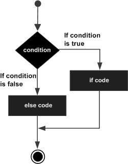
An if statement can be followed by an optional else statement, which executes when the boolean expression is false.
Syntax
The syntax of an if…else statement in C++ is −
if(boolean_expression){// statement(s) will execute if the boolean expression is true}else{// statement(s) will execute if the boolean expression is false}
If the boolean expression evaluates to true, then the if block of code will be executed, otherwise else block of code will be executed.
Flow Diagram
Example
#include <iostream>usingnamespace std;intmain(){// local variable declaration:int a =100;// check the boolean conditionif( a <20){// if condition is true then print the following
      cout <<"a is less than 20;"<< endl;}else{// if condition is false then print the following
      cout <<"a is not less than 20;"<< endl;}
   cout <<"value of a is : "<< a << endl;return0;}
When the above code is compiled and executed, it produces the following result −
a is not less than 20;
value of a is : 100
if…else if…else Statement
An if statement can be followed by an optional else if…else statement, which is very usefull to test various conditions using single if…else if statement.
When using if , else if , else statements there are few points to keep in mind.
An if can have zero or one else’s and it must come after any else if’s.
An if can have zero to many else if’s and they must come before the else.
Once an else if succeeds, none of he remaining else if’s or else’s will be tested.
Syntax
The syntax of an if…else if…else statement in C++ is −
if(boolean_expression 1){// Executes when the boolean expression 1 is true}elseif( boolean_expression 2){// Executes when the boolean expression 2 is true}elseif( boolean_expression 3){// Executes when the boolean expression 3 is true}else{// executes when the none of the above condition is true.}
Example
#include <iostream>usingnamespace std;intmain(){// local variable declaration:int a =100;// check the boolean conditionif( a ==10){// if condition is true then print the following
      cout <<"Value of a is 10"<< endl;}elseif( a ==20){// if else if condition is true
      cout <<"Value of a is 20"<< endl;}elseif( a ==30){// if else if condition is true
      cout <<"Value of a is 30"<< endl;}else{// if none of the conditions is true
      cout <<"Value of a is not matching"<< endl;}
   cout <<"Exact value of a is : "<< a << endl;return0;}
When the above code is compiled and executed, it produces the following result −
Value of a is not matching
Exact value of a is : 100
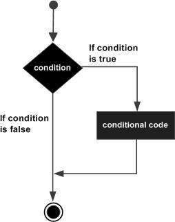
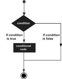
An if statement consists of a boolean expression followed by one or more statements.
Syntax
The syntax of an if statement in C++ is −
if(boolean_expression){// statement(s) will execute if the boolean expression is true}
If the boolean expression evaluates to true, then the block of code inside the if statement will be executed. If boolean expression evaluates to false, then the first set of code after the end of the if statement (after the closing curly brace) will be executed.
Flow Diagram
Example
#include <iostream>usingnamespace std;intmain(){// local variable declaration:int a =10;// check the boolean conditionif( a <20){// if condition is true then print the following
      cout <<"a is less than 20;"<< endl;}
   cout <<"value of a is : "<< a << endl;return0;}
When the above code is compiled and executed, it produces the following result −
Decision making structures require that the programmer specify one or more conditions to be evaluated or tested by the program, along with a statement or statements to be executed if the condition is determined to be true, and optionally, other statements to be executed if the condition is determined to be false.
Following is the general form of a typical decision making structure found in most of the programming languages −
C++ programming language provides following types of decision making statements.
Sr.No
Statement & Description
1
if statementAn if statement consists of a boolean expression followed by one or more statements.
2
if…else statementAn if statement can be followed by an optional else statement, which executes when the boolean expression is false.
3
switch statementA switch statement allows a variable to be tested for equality against a list of values.
4
nested if statementsYou can use one if or else if statement inside another if or else if statement(s).
We have covered conditional operator ? : in previous chapter which can be used to replace if…else statements. It has the following general form −
Exp1 ? Exp2 : Exp3;
Exp1, Exp2, and Exp3 are expressions. Notice the use and placement of the colon.
The value of a ? expression is determined like this: Exp1 is evaluated. If it is true, then Exp2 is evaluated and becomes the value of the entire ? expression. If Exp1 is false, then Exp3 is evaluated and its value becomes the value of the expression.
In C++, scope resolution operator is used to define a function outside the class and access the static variables of a class. It accesses the identifiers such as classes and functions and is denoted by double colon (::).
Here is the syntax of a scope resolution operator −
scope_name :: identifier
Here,
scope − It can be a class name, namespace, or, global.
identifier − The identifier can be a variable, function, type, or, constant.
Read this chapter to get a better understanding of various applications of scope resolution operator.
Application of Scope Resolution Operator
The scope resolution operator is used for multiple purposes that are mentioned below −
A namespace is used to differentiate similar functions, classes, variables, etc., with the same name available in different libraries. To access members which are defined inside a namespace, we use the scope resolution operator ‘::’.
In this example, we have used the scope resolution operator with cout to print the message.
#include <iostream>intmain(){
   std::cout <<"This message is printed using std::"<< std::endl;}
The output of the above code is as follows:
This message is printed using std::
Defining a Function Outside Class
To define a function outside the class, we use the scope resolution operator. It is used to differentiate a global function from a function that belongs to a class. Here is an example −
In this example, we have declared a function display in the class Example. To define this function outside the class, we have used the scope resolution operator. This function displays the value of the num.
#include <iostream>usingnamespace std;classExample{int num =10;public:voiddisplay();};voidExample::display()// Defining Function outside class{
   cout <<"The value of num is: "<< num;}intmain(){
   Example obj;
   obj.display();return0;}
The output of the above code is as follows −
The value of num is: 10
Accessing Global Variable
To access a global variable that is already locally present in a function, we use the scope resolution operator with the global variable.
The following example prints the value stored inside the variable num. The ‘num’ variable is used as local as well as a global variable, and we have used the scope resolution operator to access the global variable.
#include<iostream>usingnamespace std;int num =7;intmain(){int num =3;
   cout <<"Value of local variable num is: "<< num;
   cout <<"\nValue of global variable num is: "<<::num;return0;}
The output of the above code is as follows −
Value of local variable num is: 3
Value of global variable num is: 7
Accessing static Member Variables
To access or define a static member variable, we use a scope resolution operator. The static members belongs to class and are object-independent so they must be defined outside the class. They can be accessed using a class name with the help of the scope resolution operator.
Here is an example to define and access the static member variable name. We have used a class with a scope resolution operator to access the static variable −
An iterator in C++ is used with container like vector, list, map etc. to traverse, access, and modify the container elements. To declare an iterator, we must use the scope resolution operator (::) with the container name.
In this example, we have used an iterator it to traverse and print the vector elements using (::).
The function overriding allows a derived or child class to redefine a function that is already defined in the base or parent class. We use the scope resolution operator when we want to access the function of the parent class that is also present in the child class using the child class object.
In this example, we have used the child object to print the output of the parent class function using the scope resolution operator.
#include <iostream>usingnamespace std;classParent{public:voidshow(){
        cout <<"This is Parent class show() function"<< endl;}};classChild:public Parent{public:voidshow(){
        cout <<"This is Child class show() function"<< endl;}};intmain(){
    Child child1;
    child1.show();
    child1.Parent::show();// Calling parent class function using ::}
The output of the above code is as follows −
This is Child class show() function
This is Parent class show() function
Demonstrating Inheritance
The scope resolution operator helps you to access base class members from a derived class in inheritance. You can use scope resolution operator in single and multiple inheritance but it serves different purposes in both conditions. The following examples explain different uses of scope resolution operator in single and multiple inheritance:
Example: Single Inheritance
In this example, we have used the scope resolution operator to access the base class function display() from the derived class.
#include <iostream>usingnamespace std;classBase{public:voiddisplay(){
          cout <<"Base class function called"<< endl;}};classDerived:public Base{public:voiddisplay(){
          cout <<"Derived class function called"<< endl;}voidshowBoth(){Base::display();// Base class function using SROdisplay();// derived class function}};intmain(){
     Derived d;
     d.showBoth();return0;}
Base class function called
Derived class function called
Example: Multiple Inheritance
In multiple inheritance, there can be more than one function or variable with same name in different base classes that can cause ambiguity. This can be solved using scope resolution operator. Here is an example where display() function is called using (::) to solve this ambiguity.
#include <iostream>usingnamespace std;classClassA{public:voiddisplay(){
          cout <<"Display function from ClassA"<< endl;}};classClassB{public:voiddisplay(){
          cout <<"Display function from ClassB"<< endl;}};// Multiple InheritanceclassClassC:public ClassA, public ClassB{public:voidshowAll(){ClassA::display();// Calling ClassA's display using SROClassB::display();// Calling ClassB's display using SRO}};intmain(){
   ClassC obj;
   obj.showAll();return0;}
The output of the above code is as follows −
Display function from ClassA
Display function from ClassB
Conclusion
In this chapter, we discussed about the scope resolution operator and its various applications. Like other operators, scope resolution operator can not be overloaded. The main purpose of (::) operator is to solve the ambiguity if the variable or the functions are having same name. At compile time, scope resolution operator tells compiler about the variables and functions where they are used in the code. This solves the ambiguity caused by similar names.
A unary operator is operators that act upon a single operand to produce a new value, It manipulates or modifies only the single operand or value. It is used to perform operations like incrementing, negating, or changing the sign of a value.
The term “unary” is derived as these operators require only one operand to perform an operation. Which makes it different from binary operators, that requires two operands to perform.
This operator reverses the meaning of its operand. The operand must be of arithmetic or pointer type (or an expression that evaluates to arithmetic or pointer type). The operand is implicitly converted to type bool.
It operates on a pointer variable and returns an l-value equivalent to the value at the pointer address. Which is also called dereferencing the pointer.
It is a memory allocation operator that is used to deallocate memory that was dynamically allocated.
delete ptr;
Frees the memory allocated
Unary Arithmetic Operators in C++
In C++, Unary arithmetic operators, are the operators, that operate on a single operand to perform arithmetic operations like changing signs, incrementing, or decrementing.
Here is the following list of unary arithmetic operators in C++:
Unary Plus (+)
Unary Minus (-)
Increment (++)
Decrement (–)
Unary Plus (+) Operator
This operator doesn’t change the value of the operand, it just simply returns the operand as it is, whether the operand is negative or positive.
Syntax
+operand;
Example Code
#include <iostream>usingnamespace std;intmain(){int x =5;int y =-4;
    cout <<"Returning values using Unary plus"<< endl;
    cout <<+x <<" "<<+y << endl;return0;}
When the above code is compiled and executed, it produces the following result −
Returning values using Unary plus
5 -4
Unary Minus (-) Operator
The Unary minus or Unary negation operator is used to change the sign of the operand. If the operand is negative, it will become positive, and vice versa, where the operand can have any arithmetic type.
Syntax
-operand;
Example Code
#include usingnamespace std;intmain(){int x =6;int y =-12;
    cout <<-x <<" "<<-y << endl;return0;}
When the above code is compiled and executed, it produces the following result −
-6 12
Increment (++) Operator
The increment operator in C++ is used to increase the value of the operand by one. It has two forms:
Prefix increment (++x): First increases the value of the operand, then assigns the new value.
Postfix increment (x++): First assigns the value, then increments the operand.
Syntax for Prefix increment
++operand;
Syntax for Postfix increment
operand++;
Example Code
#include <iostream>usingnamespace std;intmain(){int x =5;// Prefix incrementint y =++x;// x is incremented first, then assigned to y
    cout <<"Prefix increment:"<< endl;
    cout <<"x = "<< x <<", y = "<< y << endl;int a =5;// Postfix incrementint b = a++;// b is assigned the value of a first, then a is incremented
    cout <<"Postfix increment:"<< endl;
    cout <<"a = "<< a <<", b = "<< b << endl;return0;}
When the above code is compiled and executed, it produces the following result −
Prefix increment:
x = 6, y = 6
Postfix increment:
a = 6, b = 5
Decrement (–) Operator
The decrement operator in C++ is used to decrement the value of an operand by one and also has two forms:
Prefix decrement (–x): First decreases the value of the operand, then assigns the new value.
Postfix decrement (x–): First assigns the value, then decrements the operand.
Syntax for Prefix decrement
--operand;
Syntax for Postfix decrement
operand--;
Example Code
#include <iostream>usingnamespace std;intmain(){int x =5;int y =--x;// First, x is decremented to 4, then assigned to y
    cout <<"x = "<< x <<" y = "<< y << endl;int a =5;int b = a--;// First, a is assigned to b, then decremented to 4
    cout <<"a = "<< a <<" b = "<< b << endl;return0;}
When the above code is compiled and executed, it produces the following result −
x = 4 y = 4
a = 4 b = 5
Unary Logical Operators
Unary logical operators in C++, are operators which deal with Boolean values, here it reverses the meaning of their operand. The operand must be of arithmetic or pointer type (or an expression that evaluates to arithmetic or pointer type). Here the operand is implicitly converted to type bool.
Syntax
!operand;
Example Code
#include <iostream>usingnamespace std;intmain(){int x =10;// non-zero value, considered Trueint y =0;// zero, considered False

    cout <<"!x = "<<!x << endl;// x is True, so !x will become false (0)
    cout <<"!y = "<<!y << endl;// y is False, so !y will become true (1)return0;}
When the above code is compiled and executed, it produces the following result −
!x = 0
!y = 1
Bitwise NOT Operator (~)
Unary bitwise NOT also known as a bitwise complement or one’s complement operator in C++ is used to perform bit-level operations. This manipulates and operates on individual bits of a variable, and produces the bitwise one’s complement of its operand. The operand must be of integral type.
Syntax
~operand;
Example Code
#include <iostream>usingnamespace std;intmain(){int x =5;// In binary: 0000000000000101 (16-bit representation)// Applying the Unary Bitwise NOT (~) operatorint result =~x;// Output the result
    cout <<"x = "<< x << endl;
    cout <<"~x = "<< result << endl;return0;}
When the above code is compiled and executed, it produces the following result −
x = 5
~x = -6
Explanation
Firstly, x is assigned the value 5, in binary 5 is represented as 0000000000000101 (16-bit signed integer representation). Applying the Unary Bitwise NOT (~) operator flips each bit of the operand, where 0 becomes 1 and 1 becomes 0.
x = 5 => 0000000000000101 (binary of 5)
~x = -6 => 1111111111111010 (bitwise complement of 5)
When working with signed integers in two’s complement, the most significant bit (leftmost bit) determines the sign of the number.
When it’s 0, the number is positive.
When it’s 1, the number is negative.
So, The binary number 1111111111111010 will give a negative decimal number. Now, to check its decimal number, add 1, which equals 0000000000000110. So, the result is -6.
Pointer Operators
Pointer operators are used to work with pointers in C++, these two pointer operators come under unary because it operates only in single operands.
Dereference (*) Operator
Dereference also known as an Indirection operator, operates on a pointer variable, which accesses the value stored at the address by a pointer and returns the value of the object that the pointer is pointing to.
Syntax
*pointer;
Address-of (&) Operator
Whereas, the Address-of operator returns the memory address of a variable. It returns the address memory where that variable is located.
Syntax
&operand;
Example Code
#include <iostream>usingnamespace std;intmain(){int num =10;// Using the Address-of operator to get the address of numint* ptr = #  // ptr now holds the address of num// Using the Dereference operator to access the value stored at
    cout <<"The value of num: "<< num << endl;
    cout <<"The address of num: "<<&num << endl;
    cout <<"The address stored in ptr: "<< ptr << endl;
    cout <<"The value pointed to by ptr: "<<*ptr << endl;return0;}
When the above code is compiled and executed, it produces the following result −
The value of num: 10
The address of num: 0x7fff08fa2814
The address stored in ptr: 0x7fff08fa2814
The value pointed to by ptr: 10
Typecast Operator (C++ Style)
The Typecast operator in C++ is a method used for explicit conversion of one data type into another.
Here, C++ provides several methods for type casting, including C and C++-style casts:
static_cast: It is used for conversion between related types (e.g. int to float, float to double, char to int, and derived class to base class).
dynamic_cast: It is used for downcasting in polymorphic class hierarchies, with runtime checking.
const_cast: It is used to add/remove the const qualifier.
reinterpret_cast: It is used for low-level pointer conversions.
Syntax
(type)operand;// C-style cast
Example Code
#include <iostream>usingnamespace std;intmain(){double a =10.78;// C-style cast: Convert double to int (fractional part is discarded)int b =(int)a;
    cout <<"Original value of a = "<< a << endl;
    cout <<"After C-style cast = "<< b << endl;return0;}
When the above code is compiled and executed, it produces the following result −
Original value of a = 10.78
After C-style cast = 10
Sizeof Operator
The sizeof operator in C++ is used to determine the size(in bytes) of any data type, variable, or data structure. It is a compile-time unary operator. This is often used for finding the memory consumption of data types, calculating the size of arrays or structures, and allocating memory dynamically using malloc or new.
Syntax
sizeof(type);
Example Code
#include <iostream>usingnamespace std;intmain(){int a =10;double b =5.75;char c ='X';// Display the size of each data type and variable
    cout <<"Size of int: "<<sizeof(a)<<" bytes"<< endl;
    cout <<"Size of double: "<<sizeof(b)<<" bytes"<< endl;
    cout <<"Size of char: "<<sizeof(c)<<" byte"<< endl;
    cout <<"Size of bool: "<<sizeof(true)<<" byte"<< endl;return0;}
When the above code is compiled and executed, it produces the following result −
Size of int: 4 bytes
Size of double: 8 bytes
Size of char: 1 byte
Size of bool: 1 byte
Type-Specific Operators
Type-Specific Operators in C++, are the operators, which is used for dynamic memory allocation and deallocation.
new: This is used to allocate memory for any single object or an array of objects.
delete: This is used to deallocate the memory allocated with new.
Syntax for new Operator
// Single object
pointer =new type;//Array of objects
pointer =new type[size];
Syntax for delete Operator
// Single objectdelete pointer;//Array of objectsdelete[] pointer;
Example Code
#include <iostream>usingnamespace std;intmain(){int* ptr =newint;*ptr =25;
    cout <<"Dynamically allocated integer: "<<*ptr << endl;// Deallocate the memory using deletedelete ptr;return0;}
When the above code is compiled and executed, it produces the following result −
The operator precedence determines the order in which operations are performed in an expression. Operators with higher precedence are evaluated first.
Example
Consider the following expression:
int x =10+4*3;
Here, the multiplication has higher precedence than addition, so 4 * 3 is evaluated first, resulting in x = 10 + 12, which gives x = 22.
To change the order, use parentheses:
int x =(10+4)*3;
Now 10 + 4 is evaluated first, resulting in x = 14 * 3, which gives x = 42.
C++ Operator Precedence Table
The operators are listed from top to bottom in descending order of precedence:
Operator
Description
Example
() [] -> .
Function call, Subscript, Member access
arr[0], obj.method(), ptr->member
++ —
Increment/Decrement
x++, –y
! ~ – +
Logical/Bitwise NOT, Unary plus/minus
!flag, ~num, -value, +value
* / %
Multiplication, Division, Modulus
a * b, x / y, n % 2
+ –
Addition, Subtraction
a + b, x – y
<< >>
Bitwise shift
x > 3
< <= > >=
Relational operators
a = y
== !=
Equality operators
a == b, x != y
&
Bitwise AND
a & b
^
Bitwise XOR
x ^ y
|
Bitwise OR
a | b
&&
Logical AND
x && y
||
Logical OR
a || b
?:
Ternary conditional
x ? y : z
= += -= *= /= %= &= ^= |= >=
Assignment and compound assignment
a = b, x += y, z >>= 2
,
Comma
x = (a, b, c)
Example of Operators Precedence
Try the following example to understand operators precedence concept available in C++. Copy and paste the following C++ program in test.cpp file and compile and run this program.
Check the simple difference with and without parenthesis. This will produce different results because (), /, * and + have different precedence. Higher precedence operators will be evaluated first −
#include <iostream>usingnamespace std;intmain(){int a =20;int b =10;int c =15;int d =5;int e;

   e =(a + b)* c / d;// ( 30 * 15 ) / 5
   cout <<"Value of (a + b) * c / d is :"<< e << endl ;

   e =((a + b)* c)/ d;// (30 * 15 ) / 5
   cout <<"Value of ((a + b) * c) / d is  :"<< e << endl ;

   e =(a + b)*(c / d);// (30) * (15/5)
   cout <<"Value of (a + b) * (c / d) is  :"<< e << endl ;

   e = a +(b * c)/ d;//  20 + (150/5)
   cout <<"Value of a + (b * c) / d is  :"<< e << endl ;return0;}
When the above code is compiled and executed, it produces the following result −
Value of (a + b) * c / d is :90
Value of ((a + b) * c) / d is  :90
Value of (a + b) * (c / d) is  :90
Value of a + (b * c) / d is  :50
C++ provides two pointer operators, which are (a) Address of Operator & and (b) Indirection Operator *.
A pointer is a variable that contains the address of another variable or you can say that a variable that contains the address of another variable is said to “point to” the other variable. A variable can be any data type including an object, structure or again pointer itself.
The . (dot) operator and the -> (arrow) operator are used to reference individual members of classes, structures, and unions.
The Address of Operator &
The & is a unary operator that returns the memory address of its operand. For example, if var is an integer variable, then &var is its address. This operator has the same precedence and right-to-left associativity as the other unary operators.
You should read the & operator as “the address of” which means &var will be read as “the address of var”.
The Indirection Operator *
The second operator is indirection Operator *, and it is the complement of &. It is a unary operator that returns the value of the variable located at the address specified by its operand.
The following program executes the two operations
#include <iostream>usingnamespace std;intmain(){int  var;int*ptr;int  val;

   var =3000;// take the address of var
   ptr =&var;// take the value available at ptr
   val =*ptr;
   cout <<"Value of var :"<< var << endl;
   cout <<"Value of ptr :"<< ptr << endl;
   cout <<"Value of val :"<< val << endl;return0;}
When the above code is compiled and executed, it produces the following result −
Value of var :3000
Value of ptr :0xbff64494
Value of val :3000
A cast is a special operator that forces one data type to be converted into another. As an operator, a cast is unary and has the same precedence as any other unary operator.
Syntax
The most general cast supported by most of the C++ compilers is as follows −
(type) expression
C++ Type Casting Operators
Where type is the desired data type. There are other casting operators supported by C++, they are listed below −
const_cast<type> (expr) − The const_cast operator is used to explicitly override const and/or volatile in a cast. The target type must be the same as the source type except for the alteration of its const or volatile attributes. This type of casting manipulates the const attribute of the passed object, either to be set or removed.
dynamic_cast<type> (expr) − The dynamic_cast performs a runtime cast that verifies the validity of the cast. If the cast cannot be made, the cast fails and the expression evaluates to null. A dynamic_cast performs casts on polymorphic types and can cast a A* pointer into a B* pointer only if the object being pointed to actually is a B object.
reinterpret_cast<type> (expr) − The reinterpret_cast operator changes a pointer to any other type of pointer. It also allows casting from pointer to an integer type and vice versa.
static_cast<type> (expr) − The static_cast operator performs a nonpolymorphic cast. For example, it can be used to cast a base class pointer into a derived class pointer.
Example of Casting Operators
All of the above-mentioned casting operators will be used while working with classes and objects. For now, try the following example to understand a simple cast operators available in C++. Copy and paste the following C++ program in test.cpp file and compile and run this program.
#include <iostream>usingnamespace std;main(){double a =21.09399;float b =10.20;int c ;

   c =(int) a;
   cout <<"Line 1 - Value of (int)a is :"<< c << endl ;

   c =(int) b;
   cout <<"Line 2 - Value of (int)b is  :"<< c << endl ;return0;}
When the above code is compiled and executed, it produces the following result −
Line 1 - Value of (int)a is :21
Line 2 - Value of (int)b is  :10
The . (dot) operator and the -> (arrow) operator are used to reference individual members of classes, structures, and unions.
The dot operator is applied to the actual object. The arrow operator is used with a pointer to an object. For example, consider the following structure −
structEmployee{char first_name[16];int age;} emp;
The (.) dot operator
To assign the value “zara” to the first_name member of object emp, you would write something as follows −
strcpy(emp.first_name,"zara");
Example
#include <iostream>#include <cstring>usingnamespace std;structEmployee{char first_name[20];};intmain(){
    Employee emp;// Using dot operator to assign a valuestrcpy(emp.first_name,"zara");

    cout <<"First Name: "<< emp.first_name << endl;return0;}
When executed, this program outputs:
First Name: zara
The (->) arrow operator
If p_emp is a pointer to an object of type Employee, then to assign the value “zara” to the first_name member of object emp, you would write something as follows −
strcpy(p_emp->first_name,"zara");
The -> is called the arrow operator. It is formed by using the minus sign followed by a greater than sign.
Example
#include <iostream>#include <cstring>usingnamespace std;structEmployee{char first_name[20];};intmain(){
    Employee emp;
    Employee* p_emp =&emp;// Using arrow operator to assign a valuestrcpy(p_emp->first_name,"zara");

    cout <<"First Name: "<< p_emp->first_name << endl;return0;}
When executed, this program outputs:
First Name: zara
Simply saying: To access members of a structure, use the dot operator. To access members of a structure through a pointer, use the arrow operator.