Author: admin

  • Maximum Bipartite Matching

    maximum bipartite graph is a type of bipartite graph that has the highest possible number of edges between two sets of vertices.

    bipartite graph is a graph where the set of vertices can be divided into two groups, such that no two vertices within the same group are directly connected. The maximum bipartite graph is one where every vertex in the first group is connected to every vertex in the second group.

    If one group has m vertices and the other has n vertices, the total number of edges in the maximum bipartite graph is:

    Emax = m  n
    

    Properties of Maximum Bipartite Graphs

    Maximum bipartite graphs have the following properties:

    • It has two separate groups of vertices, and edges only connect vertices from different groups.
    • The total number of edges is the maximum possible, which is the product of the number of vertices in each group.
    • Since there are no connections within the same group, it never contains odd-length cycles.
    • The graph can always be colored using just two colorsone for each group of vertices.
    • Maximum bipartite graphs are useful in real-world applications like job assignmentsnetworking, and resource allocation.

    Example of Maximum Bipartite Graph

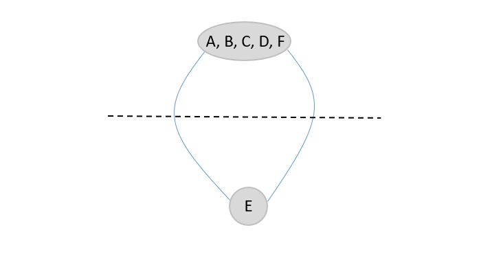
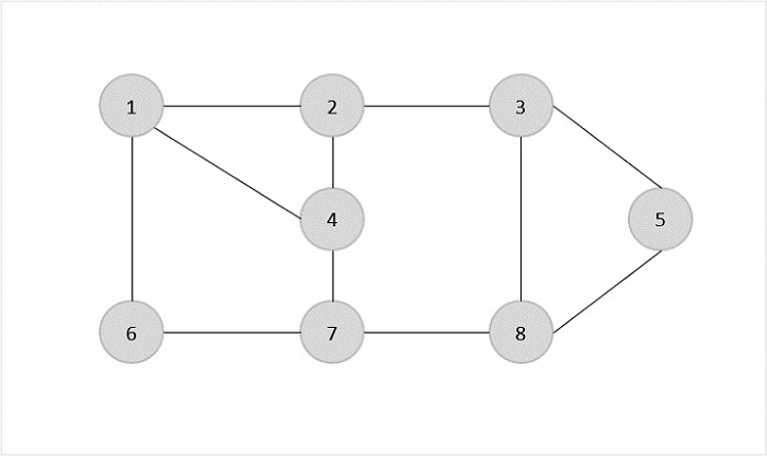
    Consider the following bipartite graph with four vertices:

    A -- B
    |    |
    C -- D
    

    In this example, the graph has two groups of vertices: {A, C} and {B, D}. The maximum bipartite graph would have the following edges:

    • A — B
    • A — D
    • C — B
    • C — D

    There are four edges in total, which is the maximum possible for this graph.

    Algorithms for Maximum Bipartite Matching

    There are several algorithms to find the maximum bipartite matching in a graph:

    • Hopcroft-Karp Algorithm
    • Ford-Fulkerson Algorithm
    • Hungarian Algorithm
    • Edmonds-Karp Algorithm
    • Augmenting Path Algorithm
    • Network Flow Algorithm

    Code to Find Maximum Bipartite Matching using Hopcroft-Karp Algorithm

    Now, let’s look at the steps to find the maximum bipartite matching in a graph using the Hopcroft-Karp algorithm:

    1. Create a bipartite graph with two sets of vertices.
    2. Initialize an empty matching between the two sets.
    3. While there is an augmenting path in the graph:
        a. Find an augmenting path using a matching algorithm.
        b. Update the matching by adding or removing edges along the path.
    4. Return the maximum matching found.
    

    Let’s look at an example of code to find the maximum bipartite matching in a graph using the Hopcroft-Karp algorithm:

    CC++JavaPython

    // C program to find maximum matching in a bipartite graph#include <stdio.h>#include <stdbool.h>#define M 6#define N 6
    
    bool bpm(int bpGraph[M][N],int u, bool seen[],int matchR[]){for(int v =0; v < N; v++){if((bpGraph[u][v]&&!seen[v])){
             seen[v]= true;if((matchR[v]<0||bpm(bpGraph, matchR[v], seen, matchR))){
                matchR[v]= u;return true;}}}return false;}intmaxBPM(int bpGraph[M][N]){int matchR[N];for(int i =0; i < N; i++)
          matchR[i]=-1;int result =0;for(int u =0; u < M; u++){
          bool seen[N];for(int i =0; i < N; i++)
             seen[i]= false;if(bpm(bpGraph, u, seen, matchR))
             result++;}return result;}intmain(){int bpGraph[M][N]={{0,1,1,0,0,0},{1,0,0,1,0,0},{0,0,1,0,0,0},{0,0,1,1,0,0},{0,0,0,0,0,0},{0,0,0,0,0,1}};printf("Maximum matching is %d\n",maxBPM(bpGraph));return0;}

    Output

    Maximum matching is 5
    

    Applications of Maximum Bipartite Matching

    Maximum bipartite matching algorithms have several real-world applications:

    • Job Assignments: Assigning tasks to workers based on their skills and availability.
    • Networking: Routing data packets through a network to optimize traffic flow.
    • Resource Allocation: Allocating resources like time, money, or equipment to maximize efficiency.
    • Marriage Matching: Pairing individuals based on preferences and compatibility.
    • Project Planning: Scheduling tasks and dependencies to complete projects on time.

    These applications demonstrate the importance of maximum bipartite matching algorithms in solving complex optimization problems.

    Time Complexity of Maximum Bipartite Matching

    The time complexity of finding the maximum bipartite matching in a graph using the Hopcroft-Karp algorithm is O(sqrt(V) * E), where V is the number of vertices and E is the number of edges in the graph. This algorithm is efficient for sparse graphs with a large number of vertices.

    Conclusion

    In this tutorial, we learned about maximum bipartite graphs and how to find the maximum bipartite matching in a graph using various algorithms. We also explored the properties and applications of maximum bipartite graphs in real-world scenarios. By understanding these concepts, you can solve a wide range of optimization problems efficiently.

  • Bellman-Ford Algorithm

    Bellman-Ford is a popular algorithm for finding the shortest path from a starting point (or “source”) to all other points in a graph, even if some edges have negative weights. While its not as fast as Dijkstras algorithm, it has a big advantage: it can handle graphs with negative edge weights.

    How does Bellman-Ford work?

    The way the Bellman-Ford algorithm works is pretty simple. It goes through all the edges of the graph multiple times and tries to improve the shortest path estimates. It “relaxes” the edges by updating the distances until they converge to the correct values.

    It continues to do this for all edges in the graph, ensuring the optimal solution.

    So, even though it might take a bit longer than Dijkstras, its a good tool when negative weights are involved!

    Alogrithm steps for Bellman-Ford

    Heres a step-by-step guide to how the Bellman-Ford algorithm works:

    • Initialization: Start by assigning a distance of 0 to the source node and infinity () to all other nodes.
    • Relaxation: Go through all the edges of the graph and relax them. Relaxing an edge means updating the distance of the destination node if a shorter path is found.
    • Repeat: Repeat the relaxation step for all edges in the graph. Keep doing this until no more improvements can be made.
    • Negative Cycle Detection: After the relaxation step, check for negative cycles. If there are negative cycles in the graph, the algorithm will detect them and report that there is no shortest path.

    Code for Bellman-Ford Algorithm

    Consider a simple graph with vertices and edges.

        (0)
        /   \
      10     15
      /       \
    (1)---5---(3)  
      \       /
       10    10
        \   /
         (4)
           \
            10
             \
              (5)
    

    Example

    Here’s an example code snippet for the Bellman-Ford Shortest Path algorithm in C, C++, Java, and Python:

    CC++JavaPython

    #include <stdio.h>#include <stdlib.h>#include <limits.h>#define MAX_VERTICES 6int graph[MAX_VERTICES][MAX_VERTICES]={{0,10,0,15,0,0},{0,0,0,5,10,0},{0,0,0,0,0,10},{0,0,0,0,0,5},{0,0,0,0,0,10},{0,0,0,0,0,0}};voidbellman_ford(int source){int distance[MAX_VERTICES];for(int i =0; i < MAX_VERTICES; i++){
          distance[i]= INT_MAX;}
       distance[source]=0;for(int i =0; i < MAX_VERTICES -1; i++){for(int u =0; u < MAX_VERTICES; u++){for(int v =0; v < MAX_VERTICES; v++){if(graph[u][v]!=0&& distance[u]!= INT_MAX && distance[u]+ graph[u][v]< distance[v]){
                   distance[v]= distance[u]+ graph[u][v];}}}}for(int u =0; u < MAX_VERTICES; u++){for(int v =0; v < MAX_VERTICES; v++){if(graph[u][v]!=0&& distance[u]!= INT_MAX && distance[u]+ graph[u][v]< distance[v]){printf("Graph contains negative weight cycle\n");return;}}}printf("Vertex   Distance from Source\n");for(int i =0; i < MAX_VERTICES; i++){if(distance[i]== INT_MAX)printf("%d \t\t INF\n", i);elseprintf("%d \t\t %d\n", i, distance[i]);}}intmain(){bellman_ford(0);return0;}

    Output

    Following is the output of the above code:

    Vertex   Distance from Source
    0 		 0
    1 		 10
    2 		 INF
    3 		 15
    4 		 20
    5 		 20
    

    Time Complexity of Bellman-Ford Algorithm

    • The time complexity of the Bellman-Ford algorithm is O(V*E), where V is the number of vertices and E is the number of edges in the graph.
    • The algorithm goes through all the edges of the graph V-1 times, relaxing them to find the shortest path.
    • If there are no negative cycles in the graph, the algorithm will converge to the correct shortest path after V-1 iterations.

    Applications of Bellman-Ford Algorithm

    The Bellman-Ford algorithm is used in various applications, including:

    • Routing Protocols: Bellman-Ford is used in routing protocols like RIP (Routing Information Protocol) to find the shortest path in computer networks.
    • Network Optimization: Its used in network optimization problems to find the shortest path between two points in a graph.
    • Resource Allocation: Bellman-Ford is used in resource allocation problems to find the most efficient way to allocate resources.
    • Graph Analysis: Its used in graph analysis to find the shortest path between two nodes in a graph.

    Conclusion

    In this tutorial, we learned about the Bellman Ford Shortest Path algorithm. It’s code, time complexity, and applications.

  • Convert Infix expression to Postfix expression

    Infix to postfix conversion rearranges math expressions to make them easier for computers to evaluate. In infix notation, operators are between operands (e.g., “A + B”). In postfix notation, operators come after operands (e.g., “A B +”). We use a stack to convert infix to postfix, ensuring the order of operations is preserved.

    What is Infix, Postfix, and Prefix?

    Before jumping into conversion, lets understand the three common types of expressions:

    • Infix: The operator is placed between operands. Example: A + B
    • Postfix (Reverse Polish Notation): The operator comes after the operands. Example: A B +
    • Prefix (Polish Notation): The operator comes before the operands. Example: + A B

    Postfix notation is useful because it eliminates the need for parentheses and follows a simple evaluation process using stacks.

    Why Use a Stack for Conversion?

    Stacks helps us to manage the order of operations (precedence) and parentheses correctly. When scanning an infix expression, we can use a stack to store operators and pop them based on precedence. This way, we can convert infix to postfix without losing the order of operations.

    Infix to Postfix Conversion Algorithm

    The algorithm for converting an infix expression to a postfix expression using a stack is:

    Read the expression from left to right.
    1. If an operand (A-Z, 0-9) is encountered, add it directly to the output.
    2. If an operator is encountered:
       1. Pop operators from the stack to the output if they have higher or equal precedence.
       2. Push the current operator onto the stack.
    3. If an opening parenthesis ( is found, push it onto the stack.
    4. If a closing parenthesis ) is found, pop operators from the stack to the output until an opening parenthesis is encountered.
    5. After scanning the entire expression, pop any remaining operators from the stack to the output.
    

    Operator Precedence

    Operators have different levels of precedence, which determine the order of evaluation:

    • ^ (Exponentiation) Highest precedence
    • *, / (Multiplication, Division) Higher precedence
    • +, - (Addition, Subtraction) Lowest precedence

    When two operators have the same precedence, we evaluate them based on associativity. Most operators are left-to-right associative, except exponentiation, which is right-to-left.

    Example: Convert Infix to Postfix

    Let’s convert the infix expression: A + B * C

    StepScanned CharacterStackPostfix Expression
    1AA
    2++A
    3B+A B
    4*+ *A B
    5C+ *A B C
    6A B C * +

    Final Postfix Expression: A B C * +

    Evaluating Postfix Expression

    Now that we have converted infix to postfix, lets see how to evaluate it:

    • Read the postfix expression from left to right.
    • If an operand is found, push it to the stack.
    • If an operator is found, pop the last two operands from the stack, apply the operation, and push the result back.
    • Continue until the expression is fully processed. The final value in the stack is the result.

    Code for Infix to Postfix Conversion

    Now that we already know the algorithm, lets see how to implement it in C, C++, Java and Python:

    CC++JavaPython

    #include <stdio.h>#include <string.h>#include <ctype.h>#define MAX 100char stack[MAX];int top =-1;voidpush(char item){if(top ==(MAX -1))printf("Stack Overflow\n");else
          stack[++top]= item;}charpop(){if(top ==-1){printf("Stack Underflow\n");return'\0';}return stack[top--];}intprecedence(char symbol){switch(symbol){case'^':return3;case'*':case'/':return2;case'+':case'-':return1;default:return0;}}voidinfixToPostfix(char infix[],char postfix[]){int i =0, j =0;char symbol;push('(');strcat(infix,")");while(infix[i]!='\0'){
          symbol = infix[i];if(symbol ==' '){
             i++;continue;}if(symbol =='(')push(symbol);elseif(isalnum(symbol))
             postfix[j++]= symbol;elseif(symbol ==')'){while(top !=-1&& stack[top]!='(')
                postfix[j++]=pop();pop();}else{while(top !=-1&&precedence(stack[top])>=precedence(symbol))
                postfix[j++]=pop();push(symbol);}
          i++;}
       postfix[j]='\0';}intmain(){char infix[MAX]="A + B * C";char postfix[MAX];printf("Infix Expression: %s\n", infix);infixToPostfix(infix, postfix);printf("Postfix Expression: %s\n", postfix);return0;}

    Output

    Following is the output of the above code:

    Enter Infix Expression: A + B * C
    Postfix Expression: ABC*+
    

    Applications of Postfix Notation

    Following are some common applications of postfix notation:

    • Used in compilers to evaluate expressions without needing parentheses.
    • Helps in designing calculators where stack-based evaluation is required.
    • Used in Expression Trees for easy computation.

    Conclusion

    Infix notation is how we naturally write mathematical expressions, but computers prefer postfix because its easier to process. We can use stack for easy Infix to Postfix conversion. Understanding this concept is crucial for solving problems related to expression evaluation and compiler design.

  • Fisher-Yates Shuffle Algorithm

    The Fisher-Yates Shuffle algorithm shuffles a finite sequence of elements by generating a random permutation. The possibility of every permutation occurring is equally likely. The algorithm is performed by storing the elements of the sequence in a sack and drawing each element randomly from the sack to form the shuffled sequence.

    Coined after Ronald Fisher and Frank Yates, for designing the original method of the shuffle, the algorithm is unbiased. It generates all permutations in same conditions so the output achieved is nowhere influenced. However, the modern version of the Fisher-Yates Algorithm is more efficient than that of the original one.

    Fisher-Yates Algorithm

    The Original Method

    The original method of Shuffle algorithm involved a pen and paper to generate a random permutation of a finite sequence. The algorithm to generate the random permutation is as follows −

    Step 1 − Write down all the elements in the finite sequence. Declare a separate list to store the output achieved.

    Step 2 − Choose an element i randomly in the input sequence and add it onto the output list. Mark the element i as visited.

    Step 3 − Repeat Step 2 until all the element in the finite sequence is visited and added onto the output list randomly.

    Step 4 − The output list generated after the process terminates is the random permutation generated.

    The Modern Algorithm

    The modern algorithm is a slightly modified version of the original fisher-yates shuffle algorithm. The main goal of the modification is to computerize the original algorithm by reducing the time complexity of the original method. The modern method is developed by Richard Durstenfeld and was popularized by Donald E. Knuth.

    Therefore, the modern method makes use of swapping instead of maintaining another output list to store the random permutation generated. The time complexity is reduced to O(n) rather than O(n2). The algorithm goes as follows −

    Step 1 − Write down the elements 1 to n in the finite sequence.

    Step 2 − Choose an element i randomly in the input sequence and swap it with the last unvisited element in the list.

    Step 3 − Repeat Step 2 until all the element in the finite sequence is visited and swapped.

    Step 4 − The list generated after the process terminates is the random permutation sequence.

    Pseudocode

    Shuffling is done from highest index to the lowest index of the array in the following modern method pseudocode.

    Fisher-Yates Shuffle (array of n elements):
    for i from n1 downto 1 do
       j ← random integer such that 0  j  i
       exchange a[j] and a[i]
    

    Shuffling is done from lowest index to the highest index of the array in the following modern method pseudocode.

    Fisher-Yates Shuffle (array of n elements):
    for i from 0 to n2 do
       j ← random integer such that i  j < n
       exchange a[i] and a[j]
    

    Original Method Example

    To describe the algorithm better, let us permute the the given finite sequence of the first six letters of the alphabet. Input sequence: A B C D E F.

    Step 1

    This is called the pen and paper method. We consider an input array with the finite sequence stored and an output array to store the result.

    input_sequence

    Step 2

    Choose any element randomly and add it onto the output list after marking it checked. In this case, we choose element C.

    output_list

    Step 3

    The next element chosen randomly is E which is marked and added to the output list.

    chosen_randomly_E

    Step 4

    The random function then picks the next element A and adds it onto the output array after marking it visited.

    next_element_A

    Step 5

    Then F is selected from the remaining elements in the input sequence and added to the output after marking it visited.

    F_selected

    Step 6

    The next element chosen to add onto the random permutation is D. It is marked and added to the output array.

    output_array

    Step 7

    The last element present in the input list would be B, so it is marked and added onto the output list finally.

    input_list_B

    Modern Method Example

    In order to reduce time complexity of the original method, the modern algorithm is introduced. The modern method uses swapping to shuffle the sequences for example, the algorithm works like shuffling a pack of cards by swapping their places in the original deck. Let us look at an example to understand how modern version of the Fisher-Yates algorithm works.

    Step 1

    Consider first few letters of the alphabet as an input and shuffle them using the modern method.

    modern_method

    Step 2

    Randomly choosing the element D and swapping it with the last unmarked element in the sequence, in this case F.

    swapped_output
    choosing_D

    Step 3

    For the next step we choose element B to swap with the last unmarked element E since F had been moved to Ds place after swapping in the previous step.

    choose_element_B
    choosed_element_B

    Step 4

    We next swap the element A with F, since it is the last unmarked element in the list.

    swap_A_with_F
    last_unmarked_element

    Step 5

    Then the element F is swapped with the last unmarked element C.

    F_swapped_C
    unmarked_element_C

    Step 6

    The remaining elements in the sequence could be swapped finally, but since the random function chose E as the element it is left as it is.

    chose_E
    chosed_E

    Step 7

    The remaining element C is left as it is without swapping.

    C_left
    final_output_array

    The array obtained after swapping is the final output array.

    Example

    Following are the implementations of the above approach in various programming langauges −

    CC++JavaPython

    #include <stdio.h>#include <stdlib.h>#include <time.h>// Function to perform Fisher-Yates Shuffle using the original methodvoidfisherYatesShuffle(char arr[],char n){char output[n];// Create an output array to store the shuffled elementschar visited[n];// Create a boolean array to keep track of visited elements// Initialize the visited array with zeros (false)for(char i =0; i < n; i++){
            visited[i]=0;}// Perform the shuffle algorithmfor(char i =0; i < n; i++){char j =rand()% n;// Generate a random index in the input arraywhile(visited[j]){// Find the next unvisited index
                j =rand()% n;}
            output[i]= arr[j];// Add the element at the chosen index to the output array
            visited[j]=1;// Mark the element as visited}// Copy the shuffled elements back to the original arrayfor(char i =0; i < n; i++){
            arr[i]= output[i];}}intmain(){char arr[]={'A','B','C','D','E','F'};char n =sizeof(arr)/sizeof(arr[0]);srand(time(NULL));// Seed the random number generator with the current timefisherYatesShuffle(arr, n);// Call the shuffle functionprintf("Shuffled array: ");for(char i =0; i < n; i++){printf("%c ", arr[i]);// Print the shuffled array}printf("\n");return0;}

    Output

    Shuffled array: A B F D E C 
  • Kargers Minimum Cut Algorithm

    Considering the real-world applications like image segmentation where objects that are focused by the camera need to be removed from the image. Here, each pixel is considered as a node and the capacity between these pixels is reduced. The algorithm that is followed is the minimum cut algorithm.

    Minimum Cut is the removal of minimum number of edges in a graph (directed or undirected) such that the graph is divided into multiple separate graphs or disjoint set of vertices.

    Let us look at an example for a clearer understanding of disjoint sets achieved

    disjoint_sets

    Edges {A, E} and {F, G} are the only ones loosely bonded to be removed easily from the graph. Hence, the minimum cut for the graph would be 2.

    minimum_cut

    The resultant graphs after removing the edges A → E and F → G are {A, B, C, D, G} and {E, F}.

    removing_edges

    Kargers Minimum Cut algorithm is a randomized algorithm to find the minimum cut of a graph. It uses the monte carlo approach so it is expected to run within a time constraint and have a minimal error in achieving output. However, if the algorithm is executed multiple times the probability of the error is reduced. The graph used in kargers minimum cut algorithm is undirected graph with no weights.

    Kargers Minimum Cut Algorithm

    The kargers algorithm merges any two nodes in the graph into one node which is known as a supernode. The edge between the two nodes is contracted and the other edges connecting other adjacent vertices can be attached to the supernode.

    Algorithm

    Step 1 − Choose any random edge [u, v] from the graph G to be contracted.

    Step 2 − Merge the vertices to form a supernode and connect the edges of the other adjacent nodes of the vertices to the supernode formed. Remove the self nodes, if any.

    Step 3 − Repeat the process until theres only two nodes left in the contracted graph.

    Step 4 − The edges connecting these two nodes are the minimum cut edges.

    The algorithm does not always the give the optimal output so the process is repeated multiple times to decrease the probability of error.

    Pseudocode

    Kargers_MinCut(edge, V, E):
       v = V
       while(v > 2):
          i=Random integer in the range [0, E-1]
          s1=find(edge[i].u)
          s2=find(edge[i].v)
          if(s1 != s2):
             v = v-1
             union(u, v)
       mincut=0
       for(i in the range 0 to E-1):
          s1=find(edge[i].u)
          s2=find(edge[i].v)
          if(s1 != s2):
             mincut = mincut + 1
       return mincut
    

    Example

    Applying the algorithm on an undirected unweighted graph G {V, E} where V and E are sets of vertices and edges present in the graph, let us find the minimum cut −

    undirected_unweighted

    Step 1

    Choose any edge, say A → B, and contract the edge by merging the two vertices into one supernode. Connect the adjacent vertex edges to the supernode. Remove the self loops, if any.

    merging_two_vertices

    Step 2

    Contract another edge (A, B) → C, so the supernode will become (A, B, C) and the adjacent edges are connected to the newly formed bigger supernode.

    bigger_supernode

    Step 3

    The node D only has one edge connected to the supernode and one adjacent edge so it will be easier to contract and connect the adjacent edge to the new supernode formed.

    new_supernode_formed

    Step 4

    Among F and E vertices, F is more strongly bonded to the supernode, so the edges connecting F and (A, B, C, D) are contracted.

    F_strongly_bonded_supernode

    Step 5

    Since there are only two nodes present in the graph, the number of edges are the final minimum cut of the graph. In this case, the minimum cut of given graph is 2.

    minimum_cut_graph

    The minimum cut of the original graph is 2 (E → D and E → F).

    Implementation

    Following are the implementations of the above approach in various programming langauges −

    CC++JavaPython

    #include <stdio.h>#include <stdlib.h>#include <time.h>structEdge{int u, v;};structGraph{int V;structEdge* edges;};structGraph*createGraph(int V,int E){structGraph* graph =(structGraph*)malloc(sizeof(structGraph));
        graph->V = V;
        graph->edges =(structEdge*)malloc(E *sizeof(structEdge));return graph;}intfind(int parent[],int i){if(parent[i]== i)return i;returnfind(parent, parent[i]);}voidunionSets(int parent[],int rank[],int x,int y){int xroot =find(parent, x);int yroot =find(parent, y);if(rank[xroot]< rank[yroot])
            parent[xroot]= yroot;elseif(rank[xroot]> rank[yroot])
            parent[yroot]= xroot;else{
            parent[yroot]= xroot;
            rank[xroot]++;}}intkargerMinCut(structGraph* graph){int V = graph->V;int E = V *(V -1)/2;structEdge* edges = graph->edges;int* parent =(int*)malloc(V *sizeof(int));int* rank =(int*)malloc(V *sizeof(int));for(int i =0; i < V; i++){
            parent[i]= i;
            rank[i]=0;}int v = V;while(v >2){int randomIndex =rand()% E;int u = edges[randomIndex].u;int w = edges[randomIndex].v;int setU =find(parent, u);int setW =find(parent, w);if(setU != setW){
                v--;unionSets(parent, rank, setU, setW);}
            edges[randomIndex]= edges[E -1];
            E--;}int minCut =0;for(int i =0; i < E; i++){int setU =find(parent, edges[i].u);int setW =find(parent, edges[i].v);if(setU != setW)
                minCut++;}free(parent);free(rank);return minCut;}intmain(){int V =4;int E =5;structGraph* graph =createGraph(V, E);
        graph->edges[0].u =0;
        graph->edges[0].v =1;
        graph->edges[1].u =0;
        graph->edges[1].v =2;
        graph->edges[2].u =0;
        graph->edges[2].v =3;
        graph->edges[3].u =1;
        graph->edges[3].v =3;
        graph->edges[4].u =2;
        graph->edges[4].v =3;srand(time(NULL));int minCut =kargerMinCut(graph);printf("Minimum Cut: %d\n", minCut);free(graph->edges);free(graph);return0;}

    Output

    Minimum Cut: 2
  • Randomized Quick Sort Algorithm

    Quicksort is a popular sorting algorithm that chooses a pivot element and sorts the input list around that pivot element. To learn more about quick sort, please click here.

    Randomized quick sort is designed to decrease the chances of the algorithm being executed in the worst case time complexity of O(n2). The worst case time complexity of quick sort arises when the input given is an already sorted list, leading to n(n 1) comparisons. There are two ways to randomize the quicksort −

    • Randomly shuffling the inputs: Randomization is done on the input list so that the sorted input is jumbled again which reduces the time complexity. However, this is not usually performed in the randomized quick sort.
    • Randomly choosing the pivot element: Making the pivot element a random variable is commonly used method in the randomized quick sort. Here, even if the input is sorted, the pivot is chosen randomly so the worst case time complexity is avoided.

    Randomized Quick Sort Algorithm

    The algorithm exactly follows the standard algorithm except it randomizes the pivot selection.

    Pseudocode

    partition-left(arr[], low, high)
       pivot = arr[high]
       i = low // place for swapping
       for j := low to high  1 do
          if arr[j] <= pivot then
             swap arr[i] with arr[j]
             i = i + 1
       swap arr[i] with arr[high]
       return i
    
    partition-right(arr[], low, high)
       r = Random Number from low to high
       Swap arr[r] and arr[high]
       return partition-left(arr, low, high)
    
    quicksort(arr[], low, high)
       if low < high
          p = partition-right(arr, low, high)
          quicksort(arr, low , p-1)
          quicksort(arr, p+1, high)
    

    Example

    Let us look at an example to understand how randomized quicksort works in avoiding the worst case time complexity. Since, we are designing randomized algorithms to decrease the occurrence of worst cases in time complexity lets take a sorted list as an input for this example.

    The sorted input list is 3, 5, 7, 8, 12, 15. We need to apply the quick sort algorithm to sort the list.

    sorted_input_list

    Step 1

    Considering the worst case possible, if the random pivot chosen is also the highest index number, it compares all the other numbers and another pivot is selected.

    pivot

    Since 15 is greater than all the other numbers in the list, it wont be swapped, and another pivot is chosen.

    Step 2

    This time, if the random pivot function chooses 7 as the pivot number −

    pivot_7

    Now the pivot divides the list into half so standard quick sort is carried out usually. However, the time complexity is decreased than the worst case.

    It is to be noted that the worst case time complexity of the quick sort will always remain O(n2) but with randomizations we are decreasing the occurrences of that worst case.

    Implementation

    Following are the implementations of the above approach in various programming langauges −

    CC++JavaPython

    #include <stdio.h>#include <stdlib.h>#include <time.h>// Function to swap two elementsvoidswap(int* a,int* b){int t =*a;*a =*b;*b = t;}// Function to partition the arrayintpartition_left(int arr[],int low,int high){int pivot = arr[high];int i = low;for(int j = low; j < high; j++){if(arr[j]<= pivot){swap(&arr[i],&arr[j]);
                i++;}}swap(&arr[i],&arr[high]);return i;}// Function to perform random partitionintpartition_right(int arr[],int low,int high){srand(time(NULL));int r = low +rand()%(high - low);swap(&arr[r],&arr[high]);returnpartition_left(arr, low, high);}// Recursive function for quicksortvoidquicksort(int arr[],int low,int high){if(low < high){int p =partition_right(arr, low, high);quicksort(arr, low, p -1);quicksort(arr, p +1, high);}}// Function to print the arrayvoidprintArray(int arr[],int size){for(int i =0; i < size; i++)printf("%d ", arr[i]);printf("\n");}// Driver codeintmain(){int arr[]={6,4,12,8,15,16};int n =sizeof(arr)/sizeof(arr[0]);printf("Original array: ");printArray(arr, n);quicksort(arr,0, n -1);printf("Sorted array: ");printArray(arr, n);return0;}

    Output

    Original array: 6 4 12 8 15 16 
    Sorted array: 4 6 8 12 15 16
  • Randomized Algorithms

    Randomized algorithm is a different design approach taken by the standard algorithms where few random bits are added to a part of their logic. They are different from deterministic algorithms; deterministic algorithms follow a definite procedure to get the same output every time an input is passed where randomized algorithms produce a different output every time theyre executed. It is important to note that it is not the input that is randomized, but the logic of the standard algorithm.

    Deterministic_Algorithm

    Figure 1: Deterministic Algorithm

    Unlike deterministic algorithms, randomized algorithms consider randomized bits of the logic along with the input that in turn contribute towards obtaining the output.

    Randomized_Algorithms

    Figure 2: Randomized Algorithm

    However, the probability of randomized algorithms providing incorrect output cannot be ruled out either. Hence, the process called amplification is performed to reduce the likelihood of these erroneous outputs. Amplification is also an algorithm that is applied to execute some parts of the randomized algorithms multiple times to increase the probability of correctness. However, too much amplification can also exceed the time constraints making the algorithm ineffective.

    Classification of Randomized Algorithms

    Randomized algorithms are classified based on whether they have time constraints as the random variable or deterministic values. They are designed in their two common forms − Las Vegas and Monte Carlo.

    Classification_Randomized_Algorithms
    • Las Vegas − The Las Vegas method of randomized algorithms never gives incorrect outputs, making the time constraint as the random variable. For example, in string matching algorithms, las vegas algorithms start from the beginning once they encounter an error. This increases the probability of correctness. Eg., Randomized Quick Sort Algorithm.
    • Monte Carlo − The Monte Carlo method of randomized algorithms focuses on finishing the execution within the given time constraint. Therefore, the running time of this method is deterministic. For example, in string matching, if monte carlo encounters an error, it restarts the algorithm from the same point. Thus, saving time. Eg., Kargers Minimum Cut Algorithm

    Need for Randomized Algorithms

    This approach is usually adopted to reduce the time complexity and space complexity. But there might be some ambiguity about how adding randomness will decrease the runtime and memory stored, instead of increasing; we will understand that using the game theory.

    The Game Theory and Randomized Algorithms

    The basic idea of game theory actually provides with few models that help understand how decision-makers in a game interact with each other. These game theoretical models use assumptions to figure out the decision-making structure of the players in a game. The popular assumptions made by these theoretical models are that the players are both rational and take into account what the opponent player would decide to do in a particular situation of a game. We will apply this theory on randomized algorithms.

    Zero-sum game

    The zero-sum game is a mathematical representation of the game theory. It has two players where the result is a gain for one player while it is an equivalent loss to the other player. So, the net improvement is the sum of both players status which sums up to zero.

    Randomized algorithms are based on the zero-sum game of designing an algorithm that gives lowest time complexity for all inputs. There are two players in the game; one designs the algorithm and the opponent provides with inputs for the algorithm. The player two needs to give the input in such a way that it will yield the worst time complexity for them to win the game. Whereas, the player one needs to design an algorithm that takes minimum time to execute any input given.

    For example, consider the quick sort algorithm where the main algorithm starts from selecting the pivot element. But, if the player in zero-sum game chooses the sorted list as an input, the standard algorithm provides the worst case time complexity. Therefore, randomizing the pivot selection would execute the algorithm faster than the worst time complexity. However, even if the algorithm chose the first element as pivot randomly and obtains the worst time complexity, executing it another time with the same input will solve the problem since it chooses another pivot this time.

    On the other hand, for algorithms like merge sort the time complexity does not depend on the input; even if the algorithm is randomized the time complexity will always remain the same. Hence, randomization is only applied on algorithms whose complexity depends on the input.

    Examples

    Few popular examples of the Randomized algorithms are −

    • Randomized Quick Sort Algorithm
    • Kargers Minimum Cut Algorithm
    • Fisher-Yates Shuffle Algorithm
    • The Subset Sum Problem
  • Travelling Salesman using Approximation Algorithm

    We have already discussed the travelling salesperson problem using the greedy and dynamic programming approaches, and it is established that solving the travelling salesperson problems for the perfect optimal solutions is not possible in polynomial time.

    Therefore, the approximation solution is expected to find a near optimal solution for this NP-Hard problem. However, an approximate algorithm is devised only if the cost function (which is defined as the distance between two plotted points) in the problem satisfies triangle inequality.

    The triangle inequality is satisfied only if the cost function c, for all the vertices of a triangle u, v and w, satisfies the following equation

                     c(u, w) c(u, v)+c(v, w)
    

    It is usually automatically satisfied in many applications.

    Travelling Salesperson Approximation Algorithm

    The travelling salesperson approximation algorithm requires some prerequisite algorithms to be performed so we can achieve a near optimal solution. Let us look at those prerequisite algorithms briefly −

    Minimum Spanning Tree − The minimum spanning tree is a tree data structure that contains all the vertices of main graph with minimum number of edges connecting them. We apply prims algorithm for minimum spanning tree in this case.

    Pre-order Traversal − The pre-order traversal is done on tree data structures where a pointer is walked through all the nodes of the tree in a [root left child right child] order.

    Algorithm

    Step 1 − Choose any vertex of the given graph randomly as the starting and ending point.

    Step 2 − Construct a minimum spanning tree of the graph with the vertex chosen as the root using prims algorithm.

    Step 3 − Once the spanning tree is constructed, pre-order traversal is performed on the minimum spanning tree obtained in the previous step.

    Step 4 − The pre-order solution obtained is the Hamiltonian path of the travelling salesperson.

    Pseudocode

    APPROX_TSP(G, c)
       r <- root node of the minimum spanning tree
       T <- MST_Prim(G, c, r)
       visited = {}
       for i in range V:
          H <- Preorder_Traversal(G)
          visited = {H}
    

    Analysis

    The approximation algorithm of the travelling salesperson problem is a 2-approximation algorithm if the triangle inequality is satisfied.

    To prove this, we need to show that the approximate cost of the problem is double the optimal cost. Few observations that support this claim would be as follows −

    • The cost of minimum spanning tree is never less than the cost of the optimal Hamiltonian path. That is, c(M) c(H*).
    • The cost of full walk is also twice as the cost of minimum spanning tree. A full walk is defined as the path traced while traversing the minimum spanning tree preorderly. Full walk traverses every edge present in the graph exactly twice. Thereore, c(W) = 2c(T)
    • Since the preorder walk path is less than the full walk path, the output of the algorithm is always lower than the cost of the full walk.

    Example

    Let us look at an example graph to visualize this approximation algorithm −

    approximation_algorithm

    Solution

    Consider vertex 1 from the above graph as the starting and ending point of the travelling salesperson and begin the algorithm from here.

    Step 1

    Starting the algorithm from vertex 1, construct a minimum spanning tree from the graph. To learn more about constructing a minimum spanning tree, please click here.

    constructing_minimum_spanning_tree

    Step 2

    Once, the minimum spanning tree is constructed, consider the starting vertex as the root node (i.e., vertex 1) and walk through the spanning tree preorderly.

    Rotating the spanning tree for easier interpretation, we get −

    Rotating_spanning_tree

    The preorder traversal of the tree is found to be − 1 → 2 → 5 → 6 → 3 → 4

    Step 3

    Adding the root node at the end of the traced path, we get, 1 → 2 → 5 → 6 → 3 → 4 → 1

    This is the output Hamiltonian path of the travelling salesman approximation problem. The cost of the path would be the sum of all the costs in the minimum spanning tree, i.e., 55.

    Implementation

    Following are the implementations of the above approach in various programming langauges −

    CC++JavaPython

    #include <stdio.h>#include <stdbool.h>#include <limits.h>#define V 6 // Number of vertices in the graph// Function to find the minimum key vertex from the set of vertices not yet included in MSTintfindMinKey(int key[], bool mstSet[]){int min = INT_MAX, min_index;for(int v =0; v < V; v++){if(mstSet[v]== false && key[v]< min){
             min = key[v];
             min_index = v;}}return min_index;}// Function to perform Prim's algorithm to find the Minimum Spanning Tree (MST)voidprimMST(int graph[V][V],int parent[]){int key[V];
       bool mstSet[V];for(int i =0; i < V; i++){
          key[i]= INT_MAX;
          mstSet[i]= false;}
       key[0]=0;
       parent[0]=-1;for(int count =0; count < V -1; count++){int u =findMinKey(key, mstSet);
          mstSet[u]= true;for(int v =0; v < V; v++){if(graph[u][v]&& mstSet[v]== false && graph[u][v]< key[v]){
                parent[v]= u;
                key[v]= graph[u][v];}}}}// Function to print the preorder traversal of the Minimum Spanning TreevoidprintPreorderTraversal(int parent[]){printf("The preorder traversal of the tree is found to be  ");for(int i =1; i < V; i++){printf("%d  ", parent[i]);}printf("\n");}// Main function for the Traveling Salesperson Approximation AlgorithmvoidtspApproximation(int graph[V][V]){int parent[V];int root =0;// Choosing vertex 0 as the starting and ending point// Find the Minimum Spanning Tree using Prim's AlgorithmprimMST(graph, parent);// Print the preorder traversal of the Minimum Spanning TreeprintPreorderTraversal(parent);// Print the Hamiltonian path (preorder traversal with the starting point added at the end)printf("Adding the root node at the end of the traced path ");for(int i =0; i < V; i++){printf("%d  ", parent[i]);}printf("%d  %d\n", root, parent[0]);// Calculate and print the cost of the Hamiltonian pathint cost =0;for(int i =1; i < V; i++){
          cost += graph[parent[i]][i];}// The cost of the path would be the sum of all the costs in the minimum spanning tree.printf("Sum of all the costs in the minimum spanning tree %d.\n", cost);}intmain(){// Example graph represented as an adjacency matrixint graph[V][V]={{0,3,1,6,0,0},{3,0,5,0,3,0},{1,5,0,5,6,4},{6,0,5,0,0,2},{0,3,6,0,0,6},{0,0,4,2,6,0}};tspApproximation(graph);return0;}

    Output

    The preorder traversal of the tree is found to be  0  0  5  1  2  
    Adding the root node at the end of the traced path -1  0  0  5  1  2  0  -1
    Sum of all the costs in the minimum spanning tree 13.
  • Set Cover Problem

    The set cover algorithm provides solution to many real-world resource allocating problems. For instance, consider an airline assigning crew members to each of their airplanes such that they have enough people to fulfill the requirements for the journey. They take into account the flight timings, the duration, the pit-stops, availability of the crew to assign them to the flights. This is where set cover algorithm comes into picture.

    Given a universal set U, containing few elements which are all divided into subsets. Considering the collection of these subsets as S = {S1, S2, S3, S4… Sn}, the set cover algorithm finds the minimum number of subsets such that they cover all the elements present in the universal set.

    universal_set

    As shown in the above diagram, the dots represent the elements present in the universal set U that are divided into different sets, S = {S1, S2, S3, S4, S5, S6}. The minimum number of sets that need to be selected to cover all the elements will be the optimal output = {S1, S2, S3}.

    Set Cover Algorithm

    The set cover takes the collection of sets as an input and and returns the minimum number of sets required to include all the universal elements.

    The set cover algorithm is an NP-Hard problem and a 2-approximation greedy algorithm.

    Algorithm

    Step 1 − Initialize Output = {} where Output represents the output set of elements.

    Step 2 − While the Output set does not include all the elements in the universal set, do the following −

    • Find the cost-effectiveness of every subset present in the universal set using the formula, Cost(Si)Si−Output
    • Find the subset with minimum cost effectiveness for each iteration performed. Add the subset to the Output set.

    Step 3 − Repeat Step 2 until there is no elements left in the universe. The output achieved is the final Output set.

    Pseudocode

    APPROX-GREEDY-SET_COVER(X, S)
       U = X
       OUTPUT = 
       while U  
          select Si  S which has maximum |SiU|
       U = U  S
       OUTPUT = OUTPUT {Si}
    return OUTPUT
    

    Analysis

    assuming the overall number of elements equals the overall number of sets (|X| = |S|), the code runs in time O(|X|3)

    Example

    Set_Cover_Algorithm

    Let us look at an example that describes the approximation algorithm for the set covering problem in more detail

    S1 = {1, 2, 3, 4}                cost(S1) = 5
    S2 = {2, 4, 5, 8, 10}            cost(S2) = 10
    S3 = {1, 3, 5, 7, 9, 11, 13}     cost(S3) = 20
    S4 = {4, 8, 12, 16, 20}          cost(S4) = 12
    S5 = {5, 6, 7, 8, 9}             cost(S5) = 15
    

    Step 1

    The output set, Output =

    Find the cost effectiveness of each set for no elements in the output set,

    S1 = cost(S1) / (S1  Output) = 5 / (4  0)
    S2 = cost(S2) / (S2  Output) = 10 / (5  0)
    S3 = cost(S3) / (S3  Output) = 20 / (7  0)
    S4 = cost(S4) / (S4  Output) = 12 / (5  0)
    S5 = cost(S5) / (S5  Output) = 15 / (5  0)
    

    The minimum cost effectiveness in this iteration is achieved at S1, therefore, the subset added to the output set, Output = {S1} with elements {1, 2, 3, 4}

    Step 2

    Find the cost effectiveness of each set for the new elements in the output set,

    S2 = cost(S2) / (S2  Output) = 10 / (5  4)
    S3 = cost(S3) / (S3  Output) = 20 / (7  4)
    S4 = cost(S4) / (S4  Output) = 12 / (5  4)
    S5 = cost(S5) / (S5  Output) = 15 / (5  4)
    

    The minimum cost effectiveness in this iteration is achieved at S3, therefore, the subset added to the output set, Output = {S1, S3} with elements {1, 2, 3, 4, 5, 7, 9, 11, 13}.

    Step 3

    Find the cost effectiveness of each set for the new elements in the output set,

    S2 = cost(S2) / (S2  Output) = 10 / |(5  9)|
    S4 = cost(S4) / (S4  Output) = 12 / |(5  9)|
    S5 = cost(S5) / (S5  Output) = 15 / |(5  9)|
    

    The minimum cost effectiveness in this iteration is achieved at S2, therefore, the subset added to the output set, Output = {S1, S3, S2} with elements {1, 2, 3, 4, 5, 7, 8, 9, 10, 11, 13}

    Step 4

    Find the cost effectiveness of each set for the new elements in the output set,

    S4 = cost(S4) / (S4  Output) = 12 / |(5  11)|
    S5 = cost(S5) / (S5  Output) = 15 / |(5  11)|
    

    The minimum cost effectiveness in this iteration is achieved at S4, therefore, the subset added to the output set, Output = {S1, S3, S2, S4} with elements {1, 2, 3, 4, 5, 7, 8, 9, 10, 11, 12, 13, 16, 20}

    Step 5

    Find the cost effectiveness of each set for the new elements in the output set,

    S5 = cost(S5) / (S5  Output) = 15 / |(5  14)|
    

    The minimum cost effectiveness in this iteration is achieved at S5, therefore, the subset added to the output set, Output = {S1, S3, S2, S4, S5} with elements {1, 2, 3, 4, 5, 6, 7, 8, 9, 10, 11, 12, 13, 16, 20}

    The final output that covers all the elements present in the universal finite set is, Output = {S1, S3, S2, S4, S5}.

    Implementation

    Following are the implementations of the above approach in various programming langauges −

    CC++JavaPython

    #include <stdio.h>#define MAX_SETS 100#define MAX_ELEMENTS 1000intsetCover(int X[],int S[][MAX_ELEMENTS],int numSets,int numElements,int output[]){int U[MAX_ELEMENTS];for(int i =0; i < numElements; i++){
          U[i]= X[i];}int selectedSets[MAX_SETS];for(int i =0; i < MAX_SETS; i++){
          selectedSets[i]=0;// Initialize all to 0 (not selected)}int outputIdx =0;while(outputIdx < numSets){// Ensure we don't exceed the maximum number of setsint maxIntersectionSize =0;int selectedSetIdx =-1;// Find the set Si with the maximum intersection with Ufor(int i =0; i < numSets; i++){if(selectedSets[i]==0){// Check if the set is not already selectedint intersectionSize =0;for(int j =0; j < numElements; j++){if(U[j]&& S[i][j]){
                      intersectionSize++;}}if(intersectionSize > maxIntersectionSize){
                   maxIntersectionSize = intersectionSize;
                   selectedSetIdx = i;}}}// If no set found, break from the loopif(selectedSetIdx ==-1){break;}// Mark the selected set as "selected" in the array
          selectedSets[selectedSetIdx]=1;// Remove the elements covered by the selected set from Ufor(int j =0; j < numElements; j++){
              U[j]= U[j]- S[selectedSetIdx][j];}// Add the selected set to the output
          output[outputIdx++]= selectedSetIdx;}return outputIdx;}intmain(){int X[MAX_ELEMENTS]={1,2,3,4,5,6,7,8,9,10};int S[MAX_SETS][MAX_ELEMENTS]={{1,1,0,0,0,0,0,0,0,0},{0,1,1,1,0,0,0,0,0,0},{0,0,0,1,1,1,0,0,0,0},{0,0,0,0,0,1,1,1,0,0},{0,0,0,0,0,0,0,1,1,1}};int numSets =5;int numElements =10;int output[MAX_SETS];int numSelectedSets =setCover(X, S, numSets, numElements, output);printf("Selected Sets: ");for(int i =0; i < numSelectedSets; i++){printf("%d ", output[i]);}printf("\n");return0;}

    Output

    Selected Sets: 1 2 3 4 0
  • Vertex Cover Algorithm

    Have you ever wondered about the placement of traffic cameras? That how they are efficiently placed without wasting too much budget from the government? The answer to that comes in the form of vertex-cover algorithm. The positions of the cameras are chosen in such a way that one camera covers as many roads as possible, i.e., we choose junctions and make sure the camera covers as much area as possible.

    vertex-cover of an undirected graph G = (V,E) is the subset of vertices of the graph such that, for all the edges (u,v) in the graph,u and v ∈ V. The junction is treated as the node of a graph and the roads as the edges. The algorithm finds the minimum set of junctions that cover maximum number of roads.

    It is a minimization problem since we find the minimum size of the vertex cover the size of the vertex cover is the number of vertices in it. The optimization problem is an NP-Complete problem and hence, cannot be solved in polynomial time; but what can be found in polynomial time is the near optimal solution.

    Vertex Cover Algorithm

    The vertex cover approximation algorithm takes an undirected graph as an input and is executed to obtain a set of vertices that is definitely twice as the size of optimal vertex cover.

    The vertex cover is a 2-approximation algorithm.

    Algorithm

    Step 1 − Select any random edge from the input graph and mark all the edges that are incident on the vertices corresponding to the selected edge.

    Step 2 − Add the vertices of the arbitrary edge to an output set.

    Step 3 − Repeat Step 1 on the remaining unmarked edges of the graph and add the vertices chosen to the output until theres no edge left unmarked.

    Step 4 − The final output set achieved would be the near-optimal vertex cover.

    Pseudocode

    APPROX-VERTEX_COVER (G: Graph)
    c ← { }
    E ← E[G]
    while E is not empty do
       Let (u, v) be an arbitrary edge of E
       c ← c U {u, v}
       Remove from E every edge incident on either u or v
    return c
    

    Example

    The set of edges of the given graph is −

    {(1,6),(1,2),(1,4),(2,3),(2,4),(6,7),(4,7),(7,8),(3,5),(8,5)}
    
    Vertex_Cover_Problem

    Now, we start by selecting an arbitrary edge (1,6). We eliminate all the edges, which are either incident to vertex 1 or 6 and we add edge (1,6) to cover.

    arbitrary_edge

    In the next step, we have chosen another edge (2,3) at random.

    chosen_another_edge

    Now we select another edge (4,7).

    select_another_edge

    We select another edge (8,5).

    another edge 8 to 5

    Hence, the vertex cover of this graph is {1,6,2,3,4,7,5,8}.

    Analysis

    It is easy to see that the running time of this algorithm is O(V + E), using adjacency list to represent E’.

    Implementation

    Following are the implementations of the above approach in various programming langauges −

    CC++JavaPython

    #include <stdio.h>#include <stdbool.h>#define MAX_VERTICES 100int graph[MAX_VERTICES][MAX_VERTICES];
    bool included[MAX_VERTICES];// Function to find Vertex Cover using the APPROX-VERTEX_COVER algorithmvoidapproxVertexCover(int vertices,int edges){
       bool edgesRemaining[MAX_VERTICES][MAX_VERTICES];for(int i =0; i < vertices; i++){for(int j =0; j < vertices; j++){
             edgesRemaining[i][j]= graph[i][j];}}while(edges >0){int u, v;for(int i =0; i < vertices; i++){for(int j =0; j < vertices; j++){if(edgesRemaining[i][j]){
                   u = i;
                   v = j;break;}}}
          included[u]= included[v]= true;for(int i =0; i < vertices; i++){
             edgesRemaining[u][i]= edgesRemaining[i][u]= false;
             edgesRemaining[v][i]= edgesRemaining[i][v]= false;}
          edges--;}}intmain(){int vertices =8;int edges =10;int edgesData[10][2]={{1,6},{1,2},{1,4},{2,3},{2,4},{6,7},{4,7},{7,8},{3,5},{8,5}};for(int i =0; i < edges; i++){int u = edgesData[i][0];int v = edgesData[i][1];
          graph[u][v]= graph[v][u]=1;}approxVertexCover(vertices, edges);printf("Vertex Cover: ");for(int i =1; i <= vertices; i++){if(included[i]){printf("%d ", i);}}printf("\n");return0;}

    Output

    Vertex Cover: 1 3 4 5 6 7